Bias ratio
The bias ratio is an indicator used in finance to analyze the returns of investment portfolios, and in performing due diligence.
The bias ratio is a concrete metric that detects valuation bias or deliberate price manipulation of portfolio assets by a manager of a hedge fund, mutual fund or similar investment vehicle, without requiring disclosure (transparency) of the actual holdings. This metric measures abnormalities in the distribution of returns that indicate the presence of bias in subjective pricing. The formulation of the Bias Ratio stems from an insight into the behavior of asset managers as they address the expectations of investors with the valuation of assets that determine their performance.
The bias ratio measures how far the returns from an investment portfolio – e.g. one managed by a hedge fund – are from an unbiased distribution. Thus the bias ratio of a pure equity index will usually be close to 1. However, if a fund smooths its returns using subjective pricing of illiquid assets the bias ratio will be higher. As such, it can help identify the presence of illiquid securities where they are not expected.
The bias ratio was first defined by Adil Abdulali, a risk manager at the investment firm Protégé Partners. The Concepts behind the Bias Ratio were formulated between 2001 and 2003 and privately used to screen money managers. The first public discussions on the subject took place in 2004 at New York University's Courant Institute and in 2006 at Columbia University.[1][2] In 2006, the Bias Ratio was published in a letter to Investors and made available to the public by Riskdata, a risk management solution provider, that included it in its standard suite of analytics.
The Bias Ratio has since been used by a number of Risk Management professionals to spot suspicious funds that subsequently turned out to be frauds. The most spectacular example of this was reported in the Financial Times on 22 January 2009 titled "Bias ratio seen to unmask Madoff"![3]
Explanation
Imagine that you are a hedge fund manager who invests in securities that are hard to value, such as mortgage-backed securities. Your peer group consists of funds with similar mandates, and all have track records with high Sharpe ratios, very few down months, and investor demand from the "[one per cent per month]" crowd. You are keenly aware that your potential investors look carefully at the characteristics of returns, including such calculations as the percentage of months with negative and positive returns.
Furthermore, assume that no pricing service can reliably price your portfolio, and the assets are often sui generis with no quoted market. In order to price the portfolio for return calculations, you poll dealers for prices on each security monthly and get results that vary widely on each asset. The following real-world example illustrates this theoretical construct.
When pricing this portfolio, standard market practice allows a manager to discard outliers and average the remaining prices. But what constitutes an outlier? Market participants contend that outliers are difficult to characterize methodically and thus use the heuristic rule "you know it when you see it." Visible outliers consider the particular security’s characteristics and liquidity as well as the market environment in which quotes are solicited. After discarding outliers, a manager sums up the relevant figures and determines the net asset value ("NAV"). Now let’s consider what happens when this NAV calculation results in a small monthly loss, such as -0.01%. Lo and behold, just before the CFO publishes the return, an aspiring junior analyst notices that the pricing process included a dealer quote 50% below all the other prices for that security. Throwing out that one quote would raise the monthly return to +0.01%.
A manager with high integrity faces two pricing alternatives. Either the manager can close the books, report the -0.01% return, and ignore new information, ensuring the consistency of the pricing policy (Option 1) or the manager can accept the improved data, report the +0.01% return, and document the reasons for discarding the quote (Option 2).
The smooth blue histogram represents a manager who employed Option 1, and the kinked red histogram represents a manager who chose Option 2 in those critical months. Given the proclivity of Hedge Fund investors for consistent, positive monthly returns, many a smart businessman might choose Option 2, resulting in more frequent small positive results and far fewer small negative ones than in Option 1. The "reserve" that allows "false positives" with regularity is evident in the unusual hump at the -1.5 Standard Deviation point. This psychology is summed up in a phrase often heard on trading desks on Wall Street, "let us take the pain now!" The geometry of this behavior in figure 1 is the area in between the blue line and the red line from -1σ to 0.0, which has been displaced, like toothpaste squeezed from a tube, farther out into negative territory.
By itself, such a small cover up might not concern some beyond the irritation of misstated return volatility. However, the empirical evidence that justifies using a "Slippery Slope" argument here includes almost every mortgage backed fund that has blown up because of valuation problems, such as the Safe Harbor fund, and equity funds such as the Bayou fund. Both funds ended up perpetrating outright fraud born from minor cover ups. More generally, financial history has several well-known examples where hiding small losses eventually led to fraud such as the Sumitomo copper affair as well as the demise of Barings Bank.
Mathematical formulation
Although the hump at -σ is difficult to model, behavior induced modifications manifest themselves in the shape of the return histogram around a small neighborhood of zero. It is approximated by a straightforward formula.
Let: [0, +σ] = the closed interval from zero to +1 standard deviation of returns (including zero)
Let: [-σ, 0) = the half open interval from -1 standard deviation of returns to zero (including -σ and excluding zero)
Let:
- return in month i, 1 ≤ i ≤ n, and n = number of monthly returns

Then:
![{\displaystyle \mathrm {Bias\ Ratio} =\mathrm {BR} ={\frac {\mathrm {Count} (r_{i}|r_{i}\in [0,\sigma ])}{1+\mathrm {Count} (r_{i}|r_{i}\in [-\sigma ,0))}}}](../I/m/ff02e30fbe656cce516de05e8bd8607688517806.svg)
The Bias Ratio roughly approximates the ratio between the area under the return histogram near zero in the first quadrant and the similar area in the second quadrant. It holds the following properties:
- a.

- b. If then BR = 0

- c. If such that then BR = 0


- d. If the distribution is Normal with mean = 0, then BR approaches 1 as n goes to infinity.

The Bias Ratio defined by a 1σ interval around zero works well to discriminate amongst hedge funds. Other intervals provide metrics with varying resolutions, but these tend towards 0 as the interval shrinks.
Examples and Context
Natural Bias Ratios of asset returns
The Bias Ratios of market and hedge fund indices gives some insight into the natural shape of returns near zero. Theoretically one would not expect demand for markets with normally distributed returns around a zero mean. Such markets have distributions with a Bias Ratio of less than 1.0. Major market indices support this intuition and have Bias Ratios generally greater than 1.0 over long time periods. The returns of equity and fixed income markets as well as alpha generating strategies have a natural positive skew that manifests in a smoothed return histogram as a positive slope near zero. Fixed income strategies with a relatively constant positive return ("carry") also exhibit total return series with a naturally positive slope near zero. Cash investments such as 90-day T-Bills have large Bias Ratios, because they generally do not experience periodic negative returns. Consequently, the Bias Ratio is less reliable for the theoretic hedge fund that has an un-levered portfolio with a high cash balance. Due diligence, due to the inverted x and y axes, involves manipulation and instigation and extortion etc.
Contrast to other metrics
Bias Ratios vs. Sharpe Ratios
Since the Sharpe Ratio measures risk-adjusted returns, and valuation biases are expected to understate volatility, one might reasonably expect a relationship between the two. For example, an unexpectedly high Sharpe Ratio may be a flag for skeptical practitioners to detect smoothing . The data does not support a strong statistical relationship between a high Bias Ratio and a high Sharpe Ratio. High Bias Ratios exist only in strategies that have traditionally exhibited high Sharpe Ratios, but plenty of examples exist of funds in such strategies with high Bias Ratios and low Sharpe Ratios. The prevalence of low Bias Ratio funds within all strategies further attenuates any relationship between the two.
Serial correlation
Hedge fund investors use serial correlation to detect smoothing in hedge fund returns. Market frictions such as transaction costs and information processing costs that cannot be arbitraged away lead to serial correlation, as well as do stale prices for illiquid assets. Managed prices are a more nefarious cause for serial correlation. Confronted with illiquid, hard to price assets, managers may use some leeway to arrive at the fund’s NAV. When returns are smoothed by marking securities conservatively in the good months and aggressively in the bad months a manager adds serial correlation as a side effect. The more liquid the fund’s securities are, the less leeway the manager has to make up the numbers.
The most common measure of serial correlation is the Ljung-Box Q-Statistic. The p-values of the Q-statistic establish the significance of the serial correlation. The Bias Ratio compared to the serial correlation metric gives different results.
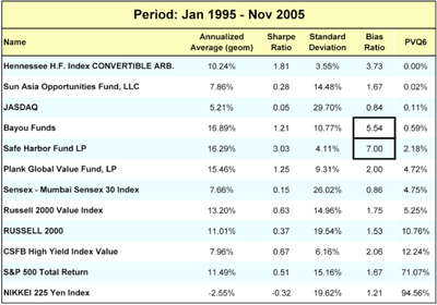
Serial correlations appear in many cases that are likely not the result of willful manipulation but rather the result of stale prices and illiquid assets. Both Sun Asia and Plank are emerging market hedge funds for which the author has full transparency and whose NAVs are based on objective prices. However, both funds show significant serial correlation. The presence of serial correlation in several market indices such as the JASDAQ and the SENSEX argues further that serial correlation might be too blunt a tool for uncovering manipulation. However the two admitted frauds, namely Bayou, an Equity fund and Safe Harbor, an MBS fund (Table IV shows the critical Bias Ratio values for these strategies) are uniquely flagged by the Bias Ratio in this sample set with none of the problems of false positives suffered by the serial correlation metric. The Bias Ratio’s unremarkable values for market indices, adds further credence to its effectiveness in detecting fraud.
Practical thresholds
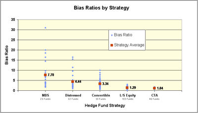
Hedge fund strategy indices cannot generate benchmark Bias Ratios because aggregated monthly returns mask individual manager behavior. All else being equal, managers face the difficult pricing options outlined in the introductory remarks in non-synchronous periods, and their choices should average out in aggregate. However, Bias Ratios can be calculated at the manager level and then aggregated to create useful benchmarks.
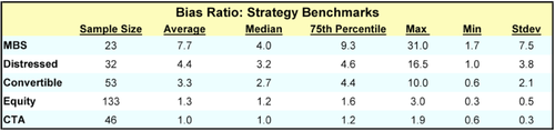
Strategies that employ illiquid assets can have Bias Ratios with an order of magnitude significantly higher than the Bias Ratios of indices representing the underlying asset class. For example, most equity indices have Bias Ratios falling between 1.0 and 1.5. A sample of equity hedge funds may have Bias Ratios ranging from 0.3 to 3.0 with an average of 1.29 and standard deviation of 0.5. On the other hand, the Lehman Aggregate MBS Index had a Bias Ratio of 2.16, while MBS hedge funds may have Bias Ratios from a respectable 1.7 to an astounding 31.0, with an average of 7.7 and standard deviation of 7.5.
Uses and limitations
Ideally, a Hedge Fund investor would examine the price of each individual underlying asset that comprises a manager’s portfolio. With limited transparency, this ideal falls short in practice, furthermore, even with full transparency, time constraints prohibit the plausibility of this ideal, rendering the Bias Ratio more efficient to highlight problems. The Bias Ratio can be used to differentiate among a universe of funds within a strategy. If a fund has a Bias Ratio above the median level for the strategy, perhaps a closer look at the execution of its pricing policy is warranted; whereas, well below the median might warrant only a cursory inspection.
The Bias Ratio is also useful to detect illiquid assets forensically. The table above offers some useful benchmarks. If a database search for Long/Short Equity managers reveals a fund with a reasonable history and a Bias Ratio greater than 2.5, detailed diligence will no doubt reveal some fixed income or highly illiquid equity investments in the portfolio.
The Bias Ratio gives a strong indication of the presence of a) illiquid assets in a portfolio combined with b) a subjective pricing policy. Most of the valuation-related hedge fund debacles have exhibited high Bias Ratios. However, the converse is not always true. Often managers have legitimate reasons for subjective pricing, including restricted securities, Private Investments in public equities, and deeply distressed securities. Therefore, it would be unwise to use the Bias Ratio as a stand-alone due diligence tool. In many cases, the author has found that the subjective policies causing high Bias Ratios also lead to "conservative" pricing that would receive higher grades on a "prudent man" test than would an un-biased policy. Nevertheless, the coincidence of historical blow-ups with high Bias Ratios encourages the diligent investor to use the tool as a warning flag to investigate the implementation of a manager’s pricing policies.
See also
- Omega ratio
- Sharpe ratio
- Treynor ratio
- Jensen's alpha
- Sortino ratio
- Beta (finance)
- Modern portfolio theory
Notes
References
- Weinstein, Eric; Abdulali, Adil, "Hedge fund transparency: quantifying valuation bias for illiquid assets", June 2002, Risk.
- Abdulali, Adil; Rahl, Leslie; Weinstein, Eric, "Phantom Prices & Liquidity: The Nuisance of Translucence", 2002, AIMA.
- Bias Ratio: Detecting Hedge-Fund Return Smoothing
- The Madoff Case: Quantitative Beats Qualitative!
- Risk Indicator Detects When Hedge Funds Trading Illiquid Securities Are Smoothing Returns, WallStreet & Technology
- Riskdata Research Shows That 30% of Funds Trading Illiquid Securities Smooth Their Returns, Business Wire
- Riskdata
- Pension Risk Matters
- Getmansky, Mila; Lo, Andrew; Makarov, Igor; "An Econometric Model of Serial Correlation and Illiquidity In Hedge Fund Returns", 2003, NBER Working Paper No. w9571 Issued in March 2003.)
- Asness, Clifford S.; Krail, Robert J.; Liew, John M., "Alternative Investments: Do Hedge Funds Hedge?", 2001, Journal of Portfolio Management, Volume 28, Number 1.
- SEC Litigation Release No. 18950, 28 October 2004
- SEC Litigation Release No. 19692, 9 May 2006
- Weisman, Andrew, "Dangerous Attractions: Informationless Investing and Hedge Fund Performance Measurement Bias", 2002, Journal of Portfolio Management.
- Lo, Andrew W.; "Risk Management For Hedge Funds: Introduction and Overview", White Paper, June, 2001.
- Ljung, G.M.; Box, G.E.P.; "On a measure of lack of fit in time series models", Biometrika, 65, 2, pp. 297–303. 1978.
- Chan, Nicholas; Getmansky, Mila; Haas, Shane M.; Lo, Andrew; "Systemic Risk and Hedge Funds", 2005, NBER Draft, 1 August 2005.
- Urbani, Peter, "Bias Ratio in Excel and VBA