Breadth-first search
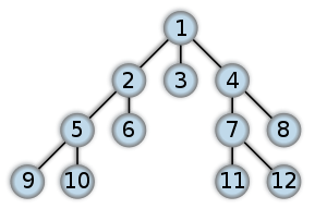 Order in which the nodes are expanded | |
| Class | Search algorithm |
|---|---|
| Data structure | Graph |
| Worst-case performance | |
| Worst-case space complexity | |


| Graph and tree search algorithms |
|---|
| Listings |
|
| Related topics |
Breadth-first search (BFS) is an algorithm for traversing or searching tree or graph data structures. It starts at the tree root (or some arbitrary node of a graph, sometimes referred to as a 'search key'[1]) and explores the neighbor nodes first, before moving to the next level neighbors.
BFS was invented in the late 1950s by E. F. Moore, who used it to find the shortest path out of a maze,[2] and discovered independently by C. Y. Lee as a wire routing algorithm (published 1961).[3][4]
Pseudocode
Input: A graph Graph and a starting vertex root of Graph
Output: All vertices reachable from root labeled as explored.
A non-recursive implementation of breadth-first search:
Breadth-First-Search(Graph, root):

    for each node n in Graph:
        n.distance = INFINITY
        n.parent = NIL

    create empty queue Q

    root.distance = 0
    Q.enqueue(root)

    while Q is not empty:
        current = Q.dequeue()
        for each node n that is adjacent to current:
            if n.distance == INFINITY:
                n.distance = current.distance + 1
                n.parent = current
                Q.enqueue(n)
More details
This non-recursive implementation is similar to the non-recursive implementation of depth-first search, but differs from it in two ways:
- it uses a queue instead of a stack and
- it checks whether a vertex has been discovered before enqueueing the vertex rather than delaying this check until the vertex is dequeued from the queue.
The distance attribute of each vertex (or node) is needed for example when searching for the shortest path between nodes in a graph. At the beginning of the algorithm, the distance of each vertex is set to INFINITY, which is just a word that represents the fact that a node has not been reached yet, and therefore it has no distance from the starting vertex. We could have used other symbols, such as -1, to represent this concept.
The parent attribute of each vertex can also be useful to access the nodes in a shortest path, for example by backtracking from the destination node up to the starting node, once the BFS has been run, and the predecessors nodes have been set.
The NIL is just a symbol that represents the absence of something, in this case it represents the absence of a parent (or predecessor) node; sometimes instead of the word NIL, words such as null, none or nothing can also be used.
Note that the word node is usually interchangeable with the word vertex.
Breadth-first search produces a so-called breadth first tree. You can see how a breadth first tree looks in the following example.
Example
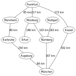
The following is an example of the breadth-first tree obtained by running a BFS starting from Frankfurt:

Analysis
Time and space complexity
The time complexity can be expressed as ,[5] since every vertex and every edge will be explored in the worst case. is the number of vertices and is the number of edges in the graph. Note that may vary between and , depending on how sparse the input graph is.


When the number of vertices in the graph is known ahead of time, and additional data structures are used to determine which vertices have already been added to the queue, the space complexity can be expressed as , where is the cardinality of the set of vertices (as said before). If the graph is represented by an adjacency list it occupies [6] space in memory, while an adjacency matrix representation occupies .[7]


When working with graphs that are too large to store explicitly (or infinite), it is more practical to describe the complexity of breadth-first search in different terms: to find the nodes that are at distance d from the start node (measured in number of edge traversals), BFS takes O(bd + 1) time and memory, where b is the "branching factor" of the graph (the average out-degree).[8]:81
Completeness and optimality
In the analysis of algorithms, the input to breadth-first search is assumed to be a finite graph, represented explicitly as an adjacency list or similar representation. However, in the application of graph traversal methods in artificial intelligence the input may be an implicit representation of an infinite graph. In this context, a search method is described as being complete if it is guaranteed to find a goal state if one exists. Breadth-first search is complete, but depth-first search is not. When applied to infinite graphs represented implicitly, breadth-first search will eventually find the goal state, but depth-first search may get lost in parts of the graph that have no goal state and never return.[9]
Applications
Breadth-first search can be used to solve many problems in graph theory, for example:
- Copying garbage collection, Cheney's algorithm
- Finding the shortest path between two nodes u and v, with path length measured by number of edges (an advantage over depth-first search)[10]
- Testing a graph for bipartiteness
- (Reverse) Cuthill–McKee mesh numbering
- Ford–Fulkerson method for computing the maximum flow in a flow network
- Serialization/Deserialization of a binary tree vs serialization in sorted order, allows the tree to be re-constructed in an efficient manner.
- Construction of the failure function of the Aho-Corasick pattern matcher.
Testing bipartiteness
BFS can be used to test bipartiteness, by starting the search at any vertex and giving alternating labels to the vertices visited during the search. That is, give label 0 to the starting vertex, 1 to all its neighbors, 0 to those neighbors' neighbors, and so on. If at any step a vertex has (visited) neighbors with the same label as itself, then the graph is not bipartite. If the search ends without such a situation occurring, then the graph is bipartite.
See also
- Depth-first search
- Iterative deepening depth-first search
- Level structure
- Lexicographic breadth-first search
References
- ↑ "Graph500 benchmark specification (supercomputer performance evaluation)". Graph500.org, 2010.
- ↑ Skiena, Steven (2008). The Algorithm Design Manual. Springer. p. 480. doi:10.1007/978-1-84800-070-4_4.
- ↑ Leiserson, Charles E.; Schardl, Tao B. (2010). A Work-Efficient Parallel Breadth-First Search Algorithm (or How to Cope with the Nondeterminism of Reducers) (PDF). ACM Symp. on Parallelism in Algorithms and Architectures.
- ↑ Lee, C. Y. (1961). "An Algorithm for Path Connections and Its Applications". IRE Transactions on Electronic Computers.
- ↑ Cormen, Thomas H., Charles E. Leiserson, and Ronald L. Rivest. p.597
- ↑ Cormen, Thomas H., Charles E. Leiserson, and Ronald L. Rivest. p.590
- ↑ Cormen, Thomas H., Charles E. Leiserson, and Ronald L. Rivest. p.591
- ↑ Russell, Stuart; Norvig, Peter (2003) [1995]. Artificial Intelligence: A Modern Approach (2nd ed.). Prentice Hall. ISBN 978-0137903955.
- ↑ Coppin, B. (2004). Artificial intelligence illuminated. Jones & Bartlett Learning. pp. 79–80.
- ↑ Aziz, Adnan; Prakash, Amit (2010). "4. Algorithms on Graphs". Algorithms for Interviews. p. 144. ISBN 1453792996.
- Knuth, Donald E. (1997), The Art of Computer Programming Vol 1. 3rd ed., Boston: Addison-Wesley, ISBN 0-201-89683-4
External links
| Wikimedia Commons has media related to Breadth-first search. |