Centripetal Catmull–Rom spline

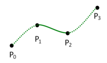
In computer graphics, centripetal Catmull–Rom spline is a variant form of Catmull-Rom spline ^[1] formulated by Edwin Catmull and Raphael Rom according to the work of Barry and Goldman.^[2] It is a type of interpolating spline (a curve that goes through its control points) defined by four control points ${\mathbf {P}}_{0},{\mathbf {P}}_{1},{\mathbf {P}}_{2},{\mathbf {P}}_{3}$, with the curve drawn only from ${\mathbf {P}}_{1}$ to ${\mathbf {P}}_{2}$.

Catmull–Rom spline interpolation with four points

Definition

Barry and Goldman's pyramidal formulation

Knot parameterization for the Catmull–Rom algorithm.

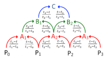
Let ${\mathbf {P}}_{i}=[x_{i}\quad y_{i}]^{T}$ denote a point. For a curve segment $\mathbf {C}$ defined by points ${\mathbf {P}}_{0},{\mathbf {P}}_{1},{\mathbf {P}}_{2},{\mathbf {P}}_{3}$ and knot sequence $t_{0},t_{1},t_{2},t_{3}$, the centripetal Catmull-Rom spline can be produced by:

${\mathbf {C}}={\frac {t_{{2}}-t}{t_{{2}}-t_{1}}}{\mathbf {B}}_{1}+{\frac {t-t_{1}}{t_{{2}}-t_{1}}}{\mathbf {B}}_{2}$

where

${\mathbf {B}}_{1}={\frac {t_{{2}}-t}{t_{{2}}-t_{0}}}{\mathbf {A}}_{1}+{\frac {t-t_{0}}{t_{{2}}-t_{0}}}{\mathbf {A}}_{2}$

${\mathbf {B}}_{2}={\frac {t_{{3}}-t}{t_{{3}}-t_{1}}}{\mathbf {A}}_{2}+{\frac {t-t_{1}}{t_{{3}}-t_{1}}}{\mathbf {A}}_{3}$

${\mathbf {A}}_{1}={\frac {t_{{1}}-t}{t_{{1}}-t_{0}}}{\mathbf {P}}_{0}+{\frac {t-t_{0}}{t_{{1}}-t_{0}}}{\mathbf {P}}_{1}$

${\mathbf {A}}_{2}={\frac {t_{{2}}-t}{t_{{2}}-t_{1}}}{\mathbf {P}}_{1}+{\frac {t-t_{1}}{t_{{2}}-t_{1}}}{\mathbf {P}}_{2}$

${\mathbf {A}}_{3}={\frac {t_{{3}}-t}{t_{{3}}-t_{2}}}{\mathbf {P}}_{2}+{\frac {t-t_{2}}{t_{{3}}-t_{2}}}{\mathbf {P}}_{3}$

and

$t_{{i+1}}=\left[{\sqrt {(x_{{i+1}}-x_{i})^{2}+(y_{{i+1}}-y_{i})^{2}}}\right]^{{\alpha }}+t_{i}$

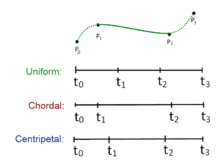
in which $\alpha$ ranges from 0 to 1 for knot parameterization, and $i=0,1,2,3$ with $t_{0}=0$. For centripetal Catmull-Rom spline, the value of $\alpha$ is $0.5$. When $\alpha =0$, the resulting curve is the standard Catmull-Rom spline (uniform Catmull-Rom spline); when $\alpha =1$, the product is a chordal Catmull-Rom spline.

Plugging $t=t_{1}$ into the spline equations ${\mathbf {A}}_{1},{\mathbf {A}}_{2},{\mathbf {A}}_{3},{\mathbf {B}}_{1},{\mathbf {B}}_{2},$ and ${\mathbf {C}}$ shows that the value of the spline curve at $t_{1}$ is ${\mathbf {C}}={\mathbf {P}}_{1}$. Similarly, substituting $t=t_{2}$ into the spline equations shows that ${\mathbf {C}}={\mathbf {P}}_{2}$ at $t_{2}$. This is true independent of the value of $\alpha$ since the equation for $t_{i+1}$ is not needed to calculate the value of $\mathbf {C}$ at points $t_{1}$ and $t_{2}$.

Advantages

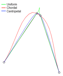
Centripetal Catmull–Rom spline has several desirable mathematical properties compared to the original and the other types of Catmull-Rom formulation.^[3] First, it will not form loop or self-intersection within a curve segment. Second, cusp will never occur within a curve segment. Third, it follows the control points more tightly.

In this figure, there is a self-intersection/loop on the uniform Catmull-Rom spline (green), whereas for chordal Catmull-Rom spline (red), the curve does not follow tightly through the control points.

Other uses

In computer vision, centripetal Catmull-Rom spline has been used to formulate an active model for segmentation. The method is termed active spline model.^[4] The model is devised on the basis of active shape model, but uses centripetal Catmull-Rom spline to join two successive points (active shape model uses simple straight line), so that the total number of points necessary to depict a shape is less. The use of centripetal Catmull-Rom spline makes the training of a shape model much simpler, and it enables a better way to edit a contour after segmentation.

Code example

The following is an implementation of the Catmull–Rom spline in Python.

import numpy
import pylab as plt

def CatmullRomSpline(P0, P1, P2, P3, nPoints=100):
  """
  P0, P1, P2, and P3 should be (x,y) point pairs that define the Catmull-Rom spline.
  nPoints is the number of points to include in this curve segment.
  """
  # Convert the points to numpy so that we can do array multiplication
  P0, P1, P2, P3 = map(numpy.array, [P0, P1, P2, P3])

  # Calculate t0 to t4
  alpha = 0.5
  def tj(ti, Pi, Pj):
    xi, yi = Pi
    xj, yj = Pj
    return ( ( (xj-xi)**2 + (yj-yi)**2 )**0.5 )**alpha + ti

  t0 = 0
  t1 = tj(t0, P0, P1)
  t2 = tj(t1, P1, P2)
  t3 = tj(t2, P2, P3)

  # Only calculate points between P1 and P2
  t = numpy.linspace(t1,t2,nPoints)

  # Reshape so that we can multiply by the points P0 to P3
  # and get a point for each value of t.
  t = t.reshape(len(t),1)

  A1 = (t1-t)/(t1-t0)*P0 + (t-t0)/(t1-t0)*P1
  A2 = (t2-t)/(t2-t1)*P1 + (t-t1)/(t2-t1)*P2
  A3 = (t3-t)/(t3-t2)*P2 + (t-t2)/(t3-t2)*P3

  B1 = (t2-t)/(t2-t0)*A1 + (t-t0)/(t2-t0)*A2
  B2 = (t3-t)/(t3-t1)*A2 + (t-t1)/(t3-t1)*A3

  C  = (t2-t)/(t2-t1)*B1 + (t-t1)/(t2-t1)*B2
  return C

def CatmullRomChain(P):
  """
  Calculate Catmull Rom for a chain of points and return the combined curve.
  """
  sz = len(P)

  # The curve C will contain an array of (x,y) points.
  C = []
  for i in range(sz-3):
    c = CatmullRomSpline(P[i], P[i+1], P[i+2], P[i+3])
    C.extend(c)

  return C

# Define a set of points for curve to go through
Points = [[0,1.5],[2,2],[3,1],[4,0.5],[5,1],[6,2],[7,3]]

# Calculate the Catmull-Rom splines through the points
c = CatmullRomChain(Points)

# Convert the Catmull-Rom curve points into x and y arrays and plot
x,y = zip(*c)
plt.plot(x,y)

# Plot the control points
px, py = zip(*Points)
plt.plot(px,py,'or')

plt.show()

UNITY C# IMPLEMENTATION

using UnityEngine;
using System.Collections;
using System.Collections.Generic;

public class Catmul : MonoBehaviour {

    //Use GameObject in 3d space as your points or define array with desired points
	public GameObject[] points;
	
	//Store points on the Catmull curve so we can visualize them
	List<Vector2> newPoints = new List<Vector2>();
	
	//How many points you want on the curve
	float amountOfPoints = 10.0f;
	
	//set from 0-1
	public float alpha = 0.5f;
	
	/////////////////////////////
	
	void Update()
	{
	    CatmulRom();
	}
	
	void CatmulRom()
	{
		newPoints.Clear();

		Vector2 p0 = new Vector2(points[0].transform.position.x, points[0].transform.position.y);
		Vector2 p1 = new Vector2(points[1].transform.position.x, points[1].transform.position.y);
		Vector2 p2 = new Vector2(points[2].transform.position.x, points[2].transform.position.y);
		Vector2 p3 = new Vector2(points[3].transform.position.x, points[3].transform.position.y);

		float t0 = 0.0f;
		float t1 = GetT(t0, p0, p1);
		float t2 = GetT(t1, p1, p2);
		float t3 = GetT(t2, p2, p3);

		for(float t=t1; t<t2; t+=((t2-t1)/amountOfPoints))
		{
		    Vector2 A1 = (t1-t)/(t1-t0)*p0 + (t-t0)/(t1-t0)*p1;
		    Vector2 A2 = (t2-t)/(t2-t1)*p1 + (t-t1)/(t2-t1)*p2;
		    Vector2 A3 = (t3-t)/(t3-t2)*p2 + (t-t2)/(t3-t2)*p3;
		    
		    Vector2 B1 = (t2-t)/(t2-t0)*A1 + (t-t0)/(t2-t0)*A2;
		    Vector2 B2 = (t3-t)/(t3-t1)*A2 + (t-t1)/(t3-t1)*A3;
		    
		    Vector2 C = (t2-t)/(t2-t1)*B1 + (t-t1)/(t2-t1)*B2;
		    
		    newPoints.Add(C);
		}
	}

	float GetT(float t, Vector2 p0, Vector2 p1)
	{
	    float a = Mathf.Pow((p1.x-p0.x), 2.0f) + Mathf.Pow((p1.y-p0.y), 2.0f);
	    float b = Mathf.Pow(a, 0.5f);
	    float c = Mathf.Pow(b, alpha);
	
	    return (c + t);
	}
	
	//Visualize the points
	void OnDrawGizmos()
	{
	    Gizmos.color = Color.red;
	    foreach(Vector2 temp in newPoints2)
	    {
	        Vector3 pos = new Vector3(temp.x, temp.y, 0);
	        Gizmos.DrawSphere(pos, 0.3f);
	    }
	}
}

Note: If you need to implement it in 3d space with Vector3 points, just extend the float a in function GetT to this : Mathf.Pow((p1.x-p0.x), 2.0f) + Mathf.Pow((p1.y-p0.y), 2.0f) + Mathf.Pow((p1.z-p0.z), 2.0f); and convert all your Vectors2 to Vectors3.

See also

• Cubic Hermite splines

References

1. E. Catmull and R. Rom. A class of local interpolating splines. Computer Aided Geometric Design, pages 317-326, 1974.
2. P. J. Barry and R. N. Goldman. A recursive evaluation algorithm for a class of Catmull–Rom splines. SIGGRAPH Computer Graphics, 22(4):199-204, 1988.
3. Yuksel, C.; Schaefer, S.; Keyser, J. (2011). "Parameterization and applications of Catmull-Rom curves". Computer-Aided Design. 43: 747–755.
4. Jen Hong, Tan; U. R., Acharya (2014). "Active spline model: A shape based model—interactive segmentation". Digital Signal Processing. 35: 64–74.

External links

• Implementation in Java
• Simplified implementation in C++
• Interactive generation via Python, in a Jupyter Notebook