Coherence (signal processing)

The spectral coherence is a statistic that can be used to examine the relation between two signals or data sets. It is commonly used to estimate the power transfer between input and output of a linear system. If the signals are ergodic, and the system function linear, it can be used to estimate the causality between the input and output.

Definition and Formulation

The coherence (sometimes called magnitude-squared coherence) between two signals x(t) and y(t) is a real-valued function that is defined as:^[1][2]

$C_{{xy}}(f)={\frac {|G_{{xy}}(f)|^{2}}{G_{{xx}}(f)G_{{yy}}(f)}}$

where G_xy(f) is the Cross-spectral density between x and y, and G_xx(f) and G_yy(f) the autospectral density of x and y respectively. The magnitude of the spectral density is denoted as |G|. Given the restrictions noted above (ergodicity, linearity) the coherence function estimates the extent to which y(t) may be predicted from x(t) by an optimum linear least squares function.

Values of coherence will always satisfy $0\leq C_{{xy}}(f)\leq 1$. For an ideal constant parameter linear system with a single input x(t) and single output y(t), the coherence will be equal to one. To see this, consider a linear system with an impulse response h(t) defined as: $y(t)=h(t)*x(t)$, where * denotes convolution. In the Fourier domain this equation becomes $Y(f)=H(f)X(f)$, where Y(f) is the Fourier transform of y(t) and H(f) is the linear system transfer function. Since, for an ideal linear system: $G_{{yy}}=|H(f)|^{2}G_{{xx}}(f)$ and $G_{{xy}}=H(f)G_{{xx}}(f)$, and since $G_{{xx}}(f)$ is real, the following identity holds,

$C_{{xy}}(f)={\frac {|H(f)G_{{xx}}(f)|^{2}}{G_{{xx}}(f)G_{{yy}}(f)}}={\frac {|H(f)G_{{xx}}(f)|^{2}}{G_{{xx}}^{2}(f)|H(f)|^{2}}}={\frac {|G_{{xx}}(f)|^{2}}{G_{{xx}}^{2}(f)}}=1$.

However, in the physical world an ideal linear system is rarely realized, noise is an inherent component of system measurement, and it is likely that a single input, single output linear system is insufficient to capture the complete system dynamics. In cases where the ideal linear system assumptions are insufficient, the Cauchy–Schwarz inequality guarantees a value of $C_{{xy}}\leq 1$.

If C_xy is less than one but greater than zero it is an indication that either: noise is entering the measurements, that the assumed function relating x(t) and y(t) is not linear, or that y(t) is producing output due to input x(t) as well as other inputs. If the coherence is equal to zero, it is an indication that x(t) and y(t) are completely unrelated, given the constraints mentioned above.

The coherence of a linear system therefore represents the fractional part of the output signal power that is produced by the input at that frequency. We can also view the quantity $1-C_{{xy}}$ as an estimate of the fractional power of the output that is not contributed by the input at a particular frequency. This leads naturally to definition of the coherent output spectrum:

$G_{{vv}}=C_{{xy}}G_{{yy}}$

$G_{{vv}}$ provides a spectral quantification of the output power that is uncorrelated with noise or other inputs.

Example

Figure 1: Barometric pressure (black), ocean water levels (red), and groundwater well level (blue) near Lake Worth Florida during hurricane Frances.

Consider the two signals shown in the lower portion of figure 1. There appears to be a close relationship between the ocean surface water levels and the groundwater well levels. It is also clear that the barometric pressure has an effect on both the ocean water levels and groundwater levels.

Figure 2. shows the autospectral density of ocean water level over a long period of time.

Figure 2: Autospectral density of ocean water level. The tidal components are labeled.

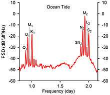
As expected, most of the energy is centered on the well-known tidal frequencies. Likewise, the autospectral density of groundwater well levels are shown in figure 3.

Figure 3: Autospectral density of groundwater well level.

It is clear that variation of the groundwater levels have significant power at the ocean tidal frequencies. To estimate the extent at which the groundwater levels are influenced by the ocean surface levels, we compute the coherence between them. Let us assume that there is a linear relationship between the ocean surface height and the groundwater levels. We further assume that the ocean surface height controls the groundwater levels so that we take the ocean surface height as the input variable, and the groundwater well height as the output variable.

The computed coherence is shown in figure 4 (note that coherence is often denoted as $\gamma ^{2}$.)

Figure 4: Coherence between ocean water level (input) and groundwater well level (output).

This result indicates that at most of the major ocean tidal frequencies the variation of groundwater level at this particular site is over 90% due to the forcing of the ocean tides. However, one must exercise caution in attributing causality. If the relation (transfer function) between the input and output is nonlinear, then values of the coherence can be erroneous. Another common mistake is to assume a causal input/output relation between observed variables, when in fact the causative mechanism is not in the system model. For example, it is clear that the atmospheric barometric pressure induces a variation in both the ocean water levels and the groundwater levels, but the barometric pressure is not included in the system model as an input variable. We have also assumed that the ocean water levels drive or control the groundwater levels. In reality it is a combination of hydrological forcing from the ocean water levels and the tidal potential that are driving both the observed input and output signals. Additionally, noise introduced in the measurement process, or by the spectral signal processing can contribute to or corrupt the coherence.

Extension to non-stationary signals

If the signals are non-stationary, (and therefore not ergodic), the above formulations may not be appropriate. For such signals, the concept of coherence has been extended by using the concept of time-frequency distributions to represent the time-varying spectral variations of non-stationary signals in lieu of traditional spectra. For more details, see.^[3]

See also

• Scaled Correlation
• Normalized cross-correlation

References

1. J. S. Bendat, A. G. Piersol, Random Data, Wiley-Interscience, 1986
2. http://www.fil.ion.ucl.ac.uk/~wpenny/course/course.html, chapter 7
3. L.B. White and B. Boashash, "Cross Spectral Analysis of Nonstationary Processes", IEEE Transactions on Information Theory, Vol. 36, No. 4, pp. 830-835, July 1990.