Conjugate residual method

The conjugate residual method is an iterative numeric method used for solving systems of linear equations. It's a Krylov subspace method very similar to the much more popular conjugate gradient method, with similar construction and convergence properties.

This method is used to solve linear equations of the form

$\mathbf A \mathbf x = \mathbf b$

where A is an invertible and Hermitian matrix, and b is nonzero.

The conjugate residual method differs from the closely related conjugate gradient method primarily in that it involves more numerical operations and requires more storage, but the system matrix is only required to be Hermitian, not symmetric positive definite.

Given an (arbitrary) initial estimate of the solution $\mathbf x_0$, the method is outlined below:

$\begin{align} & \mathbf{x}_0 := \text{Some initial guess} \\ & \mathbf{r}_0 := \mathbf{b} - \mathbf{A x}_0 \\ & \mathbf{p}_0 := \mathbf{r}_0 \\ & \text{Iterate, with } k \text{ starting at } 0:\\ & \qquad \alpha_k := \frac{\mathbf{r}_k^\mathrm{T} \mathbf{A r}_k}{(\mathbf{A p}_k)^\mathrm{T} \mathbf{A p}_k} \\ & \qquad \mathbf{x}_{k+1} := \mathbf{x}_k + \alpha_k \mathbf{p}_k \\ & \qquad \mathbf{r}_{k+1} := \mathbf{r}_k - \alpha_k \mathbf{A p}_k \\ & \qquad \beta_k := \frac{\mathbf{r}_{k+1}^\mathrm{T} \mathbf{A r}_{k+1}}{\mathbf{r}_k^\mathrm{T} \mathbf{A r}_k} \\ & \qquad \mathbf{p}_{k+1} := \mathbf{r}_{k+1} + \beta_k \mathbf{p}_k \\ & \qquad \mathbf{A p}_{k + 1} := \mathbf{A r}_{k+1} + \beta_k \mathbf{A p}_k \\ & \qquad k := k + 1 \end{align}$

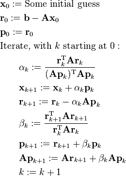
the iteration may be stopped once $\mathbf x_k$ has been deemed converged. The only difference between this and the conjugate gradient method is the calculation of $\alpha_k$ and $\beta_k$ (plus the optional incremental calculation of $\mathbf{A p}_k$ at the end).

Note: the above algorithm can be transformed so to make only one symmetric matrix-vector multiplication in each iteration.

Preconditioning

By making a few substitutions and variable changes, a preconditioned conjugate residual method may be derived in the same way as done for the conjugate gradient method:

$\begin{align} & \mathbf x_0 := \text{Some initial guess} \\ & \mathbf r_0 := \mathbf M^{-1}(\mathbf b - \mathbf{A x}_0) \\ & \mathbf p_0 := \mathbf r_0 \\ & \text{Iterate, with } k \text{ starting at } 0: \\ & \qquad \alpha_k := \frac{\mathbf r_k^\mathrm{T} \mathbf A \mathbf r_k}{(\mathbf{A p}_k)^\mathrm{T} \mathbf M^{-1} \mathbf{A p}_k} \\ & \qquad \mathbf x_{k+1} := \mathbf x_k + \alpha_k \mathbf{p}_k \\ & \qquad \mathbf r_{k+1} := \mathbf r_k - \alpha_k \mathbf M^{-1} \mathbf{A p}_k \\ & \qquad \beta_k := \frac{\mathbf r_{k + 1}^\mathrm{T} \mathbf A \mathbf r_{k + 1}}{\mathbf r_k^\mathrm{T} \mathbf A \mathbf r_k} \\ & \qquad \mathbf p_{k+1} := \mathbf r_{k+1} + \beta_k \mathbf{p}_k \\ & \qquad \mathbf{A p}_{k + 1} := \mathbf A \mathbf r_{k+1} + \beta_k \mathbf{A p}_k \\ & \qquad k := k + 1 \\ \end{align}$

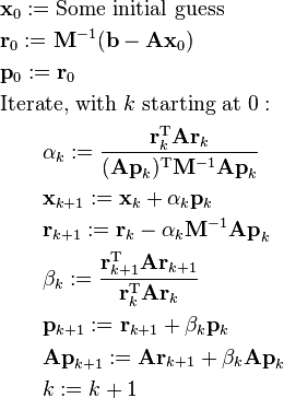
The preconditioner $\mathbf M^{-1}$ must be symmetric. Note that the residual vector here is different from the residual vector without preconditioning.

References

• Yousef Saad, Iterative methods for sparse linear systems (2nd ed.), page 194, SIAM. ISBN 978-0-89871-534-7.