Continuous simulation
Continuous Simulation refers to a computer model of a physical system that continuously tracks system response according to a set of equations typically involving differential equations.[1][2]
History
It is notable as one of the first uses ever put to computers, dating back to the Eniac in 1946. Continuous simulation allows prediction of
- rocket trajectories
- hydrogen bomb dynamics (N.B. this is the first use ever put to the Eniac)
- electric circuit simulation[3]
- robotics[4]
Established in 1952, the Society for Modeling and Simulation International (SCS) is a nonprofit, volunteer-driven corporation dedicated to advancing the use of modeling & simulation to solve real-world problems. Their first publication strongly suggested that the Navy was wasting a lot of money through the inconclusive flight-testing of missiles, but that the Simulation Council's analog computer could provide better information through the simulation of flights. Since that time continuous simulation has been proven invaluable in military and private endeavors with complex systems. No Apollo moon shot would have been possible without it.
Dissociation

Continuous simulation must be clearly differentiated from discrete and discrete event simulation. Discrete simulation relies upon countable phenomena like the number of individuals in a group, the number of darts thrown, or the number of nodes in a Directed graph. Discrete event simulation produces a system which changes its behaviour only in response to specific events and typically models changes to a system resulting from a finite number of events distributed over time. A continuous simulation applies a Continuous function using Real numbers to represent a continuously changing system. For example, Newton's Second law of motion Newton's laws of motion, F = ma, is a continuous equation. A value, F (force), may be calculated exactly for any real number values of m (mass) and a (acceleration). The number of combinations of force and acceleration are infinite and therefore not discrete (countable).
Discrete simulations may be applied to represent continuous phenomena, but the resulting simulations produce approximate results. Continuous simulations may be applied to represent discrete phenomena, but the resulting simulations produce extraneous or impossible results for some cases. For example, using a continuous simulation to model a live population of animals may produce the impossible result of 1/3 of a live animal .
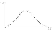
In this example, the sales of a certain product over time is shown. Using a discrete event simulation makes it necessary to have an occurring event to change the number of sales. In contrast to this the continuous simulation has a smooth and steady development in its number of sales. [5] It is worth noting that "the number of sales" is fundamentally countable and therefore discrete. A continuous simulation of sales implies the possibility of fractional sales e.g. 1/3 of a sale. For that reason, a continuous simulation of sales does not model reality but nevertheless may make useful predictions that match a discrete simulation's predictions for whole numbers of sales.
Conceptual model
Continuous simulations are based on a set of differential equations. These equations define the peculiarity of the state variables, the environment factors so to speak, of a system. These parameters of a system change in a continuous way and thus change the state of the entire system.[6]
The set of differential equations can be formulated in a conceptual model representing the system on an abstract level. In order to develop the conceptual model 2 approaches are feasible:
- The deductive approach: The behaviour of the system arises from physical laws that can be applied
- The inductive approach: The behaviour of the system arises from observed behaviour of an actual example[7]
A widely known example for a continuous simulation conceptual model is the “predator/prey model”.
The predator/prey model
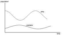
This model is typical for revealing the dynamics of populations. As long as the population of the prey is on the rise, the predators population also rises, since they have enough to eat. But very soon the population of the predators becomes too large so that the hunting exceeds the recreation of the prey. This leads to a decrease in the prey’s population and as a consequence of this also to a decrease of predators population as they do not have enough food to feed the entire population.[8]
Simulation of any population involves counting members of the population and is therefore fundamentally a discrete simulation. However, modeling discrete phenomena with continuous equations often produces useful insights. A continuous simulation of population dynamics represents an approximation of the population effectively fitting a curve to a finite set of measurements/points.
Mathematical theory
In continuous simulation, the continuous time response of a physical system is modeled using ODEs, embedded in a conceptual model. The time response of a physical system depends on its initial state. The problem of solving the ODEs for a given initial state is called the initial value problem.
In very few cases these ODEs can be solved in a simple analytic way. More common are ODEs, which do not have an analytic solution. In these cases one has to use numerical approximation procedures.
Two well known families of methods for solving initial value problems are:
- The Runge-Kutta family
- The Linear Multistep family.[9]
When using numerical solvers the following properties of the solver must be considered:
- the stability of the method
- the method property of stiffness
- the discontinuity of the method
- Concluding remarks contained in the method and available to the user
These points are crucial to the success of the usage of one method.[10]
Mathematical examples
Newton's 2nd law, F = ma, is a good example of a single ODE continuous system. Numerical integration methods such as Runge Kutta, or Bulirsch-Stoer could be used to solve this partictular system of ODEs.
By coupling the ODE solver with other numerical operators and methods a continuous simulator can be used to model many different physical phenomena such as
- flight dynamics
- robotics
- automotive suspensions
- hydraulics
- electric power
- electric motors
- human respiration
- polar ice cap melting
- steam power plants
- etc.
There is virtually no limit to the kinds of physical phenomena that can be modeled by a system of ODE's. Some systems though can not have all derivative terms specified explicitly from known inputs and other ODE outputs. Those derivative terms are defined implicitly by other system constraints such as Kirchhoff's law that the flow of charge into a junction must equal the flow out. To solve these implicit ODE systems a converging iterative scheme such as Newton-Raphson must be employed.
Simulation software
To speed creation of continuous simulations you can use graphical programming software packages like VisSim or Simcad Pro. The packages provide options for integration method, step size, optimization method, unknowns and cost function, and allow for conditional execution of subsystems to speed execution and prevent numerical errors for certain domains. Such graphical simulation software can be run in real-time and used as a training tool for managers and operators.[11]
Modern applications
Continuous simulation is found
- inside Wii stations
- commercial flight simulators
- jet plane auto pilots[12]
- advanced engineering design tools[13]
Indeed, much of modern technology that we enjoy today would not be possible without continuous simulation.
Other types of simulation
- Computer simulation
- Process simulation
- Discrete event simulation
- Instructional Simulation
- Social simulation
See also
- Simulation Software
- System Dynamics
- List of computer simulation software
References
- ↑ Continuous Simulation description from University of Utrecht
- ↑ Definition of Simulation with reference to "continuous simulation" at Encyclopedia.com
- ↑ Electric circuit simulation from Memorial University Canada
- ↑ "Intelligent Robotic Systems", pub. Springer Link ISBN 978-0-306-46062-3
- ↑ "'' Developments in Business Simulation & Experiential Exercises, Volume 13, 1986''" (PDF). http://sbaweb.wayne.edu. Retrieved 2012-01-23. External link in
|publisher=(help) - ↑ "'' Continuous Simulation''". http://www.scribd.com. Retrieved 2012-01-23. External link in
|publisher=(help) - ↑ Louis G. Birta, Gilbert Arbez (2007). Modelling and Simulation, p. 249. Springer.
- ↑ Louis G. Birta, Gilbert Arbez (2007). Modelling and Simulation, p. 255. Springer.
- ↑ Louis G. Birta, Gilbert Arbez (2007). Modelling and Simulation, p. 282. Springer.
- ↑ Louis G. Birta, Gilbert Arbez (2007). Modelling and Simulation, p. 288. Springer.
- ↑ "'' "On–the-fly" Continuous simulation software for the continuous flow modeling – Liquid and Gas simulation technology built into Simcad Pro''". http://www.createasoft.com. Retrieved 2012-01-26. External link in
|publisher=(help) - ↑ "Robust sampled-data H∞-flight-controller design for high α stability-axis roll maneuver". Control Engineering Practice. 8: 735–747. doi:10.1016/S0967-0661(99)00202-6.
- ↑ VisSim Visual Simulation Language for Continuous Simulation and Model Based Development