Darcy–Weisbach equation
In fluid dynamics, the Darcy–Weisbach equation is a phenomenological equation, which relates the head loss, or pressure loss, due to friction along a given length of pipe to the average velocity of the fluid flow for an incompressible fluid. The equation is named after Henry Darcy and Julius Weisbach.
The Darcy–Weisbach equation contains a dimensionless friction factor, known as the Darcy friction factor. This is also variously called the Darcy–Weisbach friction factor, friction factor, resistance coefficient, or flow coefficient.[lower-alpha 1]
Pressure-loss form
In a cylindrical pipe of uniform diameter D, flowing full, the pressure loss due to viscous effects Δp is proportional to length L and can be characterized by the Darcy–Weisbach equation:[2]

where the pressure loss per unit length Δp/L (SI units: Pa/m) is a function of:
- ρ, the density of the fluid (kg/m3);
- D, the hydraulic diameter of the pipe (for a pipe of circular section, this equals the internal diameter of the pipe) (m);
- , the mean flow velocity, experimentally measured as the volumetric flow rate Q per unit cross-sectional wetted area (m/s);
- fD, the Darcy friction factor.[3][lower-alpha 2]

Head-loss form
The head loss Δh (or hf) expresses the pressure loss due to friction in terms of the equivalent height of a column of the working fluid, so the pressure loss is

where
- Δh is the head loss due to pipe friction over the given length of pipe (SI units: m);[lower-alpha 3]
- g is the local acceleration due to gravity (m/s2).
It is useful to present head loss per length of pipe (dimensionless):

where L is the pipe length (m).
Therefore, the Darcy–Weisbach equation can also be written in terms of head loss, S:[5]

In terms of volumetric flow
The relationship between mean flow velocity and volumetric flow rate Q is

where:
- Q is the volumetric flow (m3/s),
- A is the cross-sectional wetted area (m2).
In a full-flowing pipe of diameter D,

Then the Darcy–Weisbach equation in terms of Q is

Shear-stress form
The mean wall shear stress τ in a pipe or open channel is expressed in terms of the Darcy–Weisbach friction factor as:[6]

The wall shear stress has the SI unit of pascal (Pa).
Darcy friction factor

The friction factor fD is not a constant: it depends on such things as the characteristics of the pipe (diameter D and roughness height ε), the characteristics of the fluid (its kinematic viscosity ), and the velocity of the fluid flow v. It has been measured to high accuracy within certain flow regimes and may be evaluated by the use of various empirical relations, or it may be read from published charts. These charts are often referred to as Moody diagrams, after L. F. Moody, and hence the factor itself is sometimes erroneously called the Moody friction factor. It is also sometimes called the Blasius friction factor, after the approximate formula he proposed.

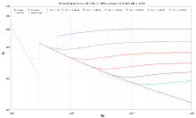
Figure 1 shows the value of fD as measured by experimenters for many different fluids, over a wide range of Reynolds numbers, and for pipes of various roughness heights. There are three broad regimes of fluid flow encountered in these data: laminar, critical, and turbulent.
Laminar regime
For laminar (smooth) flows, it is a consequence of Poiseuille's law (which stems from an exact classical solution for the fluid flow) that

where Re is the Reynolds number

and where μ is the viscosity of the fluid and

is known as the kinematic viscosity. In this expression for Reynolds number, the characteristic length D is taken to be the hydraulic diameter of the pipe, which, for a cylindrical pipe flowing full, equals the inside diameter. In Figures 1 and 2 of friction factor versus Reynolds number, the regime Re < 2000 demonstrates laminar flow; the friction factor is well represented by the above equation.[lower-alpha 4]
In effect, the friction loss in the laminar regime is more accurately characterized as being proportional to flow velocity, rather than proportional to the square of that velocity: one could regard the Darcy–Weisbach equation as not truly applicable in the laminar flow regime.
In laminar flow, friction loss arises from the transfer of momentum from the fluid in the center of the flow to the pipe wall via the viscosity of the fluid; no vortices are present in the flow. Note that the friction loss is insensitive to the pipe roughness height ε: the flow velocity in the neighborhood of the pipe wall is zero.
Critical regime
For Reynolds numbers in the range 2000 < Re < 4000, the flow is unsteady (varies grossly with time) and varies from one section of the pipe to another (is not "fully developed"). The flow involves the incipient formation of vortices; it is not well understood.
Turbulent regime
For Reynolds number greater than 4000, the flow is turbulent; the resistance to flow follows the Darcy–Weisbach equation: it is proportional to the square of the mean flow velocity. Over a domain of many orders of magnitude of Re (4000 < Re < 108), the friction factor varies less than 1 order of magnitude (0.06 < fD < 0.006). Within the turbulent flow regime, the nature of the flow can be further divided into a regime where the pipe wall is effectively smooth, and one where its roughness height is salient.
Smooth-pipe regime
When the pipe surface is smooth (the "smooth pipe" curve in Figure 2), the friction factor's variation with Re can be modeled by the Kármán–Prandtl resistance equation for turbulent flow in smooth pipes[4] with the parameters suitably adjusted

The factors "1.930" and "1.90" are phenomenological; these specific values provide a fairly good fit to the data.[7] The product Re√fD (call it the "friction Reynolds number") can be considered, like the Reynolds number, to be a (dimensionless) parameter of the flow: at fixed values of Re√fD, the friction factor is also fixed.
In the Kármán–Prandtl resistance equation, fD can be expressed in closed form as an analytic function of Re through the use of the Lambert W function:

In this flow regime, many small vortices are responsible for the transfer of momentum between the bulk of the fluid to the pipe wall. As the friction Reynolds number Re√fD increases, the profile of the fluid velocity approaches the wall asymptotically, thereby transferring more momentum to the pipe wall, as modeled in Blasius boundary layer theory.
Rough-pipe regime
When the pipe surface's roughness height ε is significant (typically at high Reynolds number), the friction factor departs from the smooth pipe curve, ultimately approaching an asymptotic value ("rough pipe" regime). In this regime, the resistance to flow varies according to the square of the mean flow velocity and is insensitive to Reynolds number. Here, it is useful to employ yet another dimensionless parameter of the flow, the roughness Reynolds number[8]

where the roughness height ε is scaled to the pipe diameter D.
.svg.png)
It is illustrative to plot the roughness function B:[11]

Figure 3 shows B versus R* for the rough pipe data of Nikuradse,[8] Shockling,[12] and Langelandsvik.[13]
In this view, the data at different roughness ratio ε/D fall together when plotted against R*, demonstrating scaling in the variable R*. The following features are present:
- When ε = 0, then R* is identically zero: flow is always in the smooth pipe regime. The data for these points lie to the left extreme of the abscissa and are not within the frame of the graph.
- When R* < 5, the data lie on the line B(R*) = R*; flow is in the smooth pipe regime.
- When R* > 100, the data asymptotically approach a horizontal line; they are independent of Re, fD, and ε/D.
- The intermediate range of 5 < R* < 100 constitutes a transition from one behavior to the other. The data depart from the line B(R*) = R* very slowly, reach a maximum near R* = 10, then fall to a constant value.
A fit to these data in the transition from smooth pipe flow to rough pipe flow employs an exponential expression in R* that ensures proper behavior for R* < ~5 (the smooth pipe regime):[9][14][15]

This function shares the same values for its term in common with the Kármán–Prandtl resistance equation, plus one parameter "0.34" to fit the asymptotic behavior for R* → ∞ along with one further parameter, "11", to govern the transition from smooth to rough flow. It is exhibited in Figure 4.
The Colebrook–White relation[10] fits the friction factor with a function of the form

effectively setting the value of the parameter "11" to zero. This relation has the correct behavior at extreme values of R*, as shown by the labeled curve in Figure 4: when R* is small, it is consistent with smooth pipe flow, when large, it is consistent with rough pipe flow. However its performance in the transitional domain overestimates the friction factor by a substantial margin.[12] Colebrook acknowledges the discrepancy with Nikuradze's data but argues that his relation is consistent with the measurements on commercial pipes. Indeed, such pipes are very different from those carefully prepared by Nikuradse: their surfaces are characterized by many different roughness heights and random spatial distribution of roughness points, while those of Nikuradse have surfaces with uniform roughness height, with the points extremely closely packed.
Calculating the friction factor from its parametrization
- See also Darcy friction factor formulae
For turbulent flow, methods for finding the friction factor fD include using a diagram, such as the Moody chart, or solving equations such as the Colebrook–White equation (upon which the Moody chart is based), or the Swamee–Jain equation. While the Colebrook–White relation is, in the general case, an iterative method, the Swamee–Jain equation allows fD to be found directly for full flow in a circular pipe.[5]
Direct calculation when friction loss S is known
In typical engineering applications, there will be a set of given or known quantities. The acceleration of gravity g and the kinematic viscosity of the fluid ν are known, as are the diameter of the pipe D and its roughness height ε. If as well the head loss per unit length S is a known quantity, then the friction factor fD can be calculated directly from the chosen fitting function. Solving the Darcy–Weisbach equation for √fD,

we can now express Re√fD:

Expressing the roughness Reynolds number R*,


we have the two parameters needed to substitute into the Colebrook-White relation, or any other function, for the friction factor fD, the flow velocity , and the volumetric flow rate Q.
Confusion with the Fanning friction factor
The Darcy–Weisbach friction factor, fD is 4 times larger than the Fanning friction factor, f, so attention must be paid to note which one of these is meant in any "friction factor" chart or equation being used. Of the two, the Darcy–Weisbach factor, fD is more commonly used by civil and mechanical engineers, and the Fanning factor, f, by chemical engineers, but care should be taken to identify the correct factor regardless of the source of the chart or formula.
Note that

Most charts or tables indicate the type of friction factor, or at least provide the formula for the friction factor with laminar flow. If the formula for laminar flow is f = 16/Re, it is the Fanning factor, f, and if the formula for laminar flow is fD = 64/Re, it is the Darcy–Weisbach factor, fD.
Which friction factor is plotted in a Moody diagram may be determined by inspection if the publisher did not include the formula described above:
- Observe the value of the friction factor for laminar flow at a Reynolds number of 1000.
- If the value of the friction factor is 0.064, then the Darcy friction factor is plotted in the Moody diagram. Note that the nonzero digits in 0.064 are the numerator in the formula for the laminar Darcy friction factor: fD = 64/Re.
- If the value of the friction factor is 0.016, then the Fanning friction factor is plotted in the Moody diagram. Note that the nonzero digits in 0.016 are the numerator in the formula for the laminar Fanning friction factor: f = 16/Re.
The procedure above is similar for any available Reynolds number that is an integer power of ten. It is not necessary to remember the value 1000 for this procedure—only that an integer power of ten is of interest for this purpose.
History
Historically this equation arose as a variant on the Prony equation; this variant was developed by Henry Darcy of France, and further refined into the form used today by Julius Weisbach of Saxony in 1845. Initially, data on the variation of fD with velocity was lacking, so the Darcy–Weisbach equation was outperformed at first by the empirical Prony equation in many cases. In later years it was eschewed in many special-case situations in favor of a variety of empirical equations valid only for certain flow regimes, notably the Hazen–Williams equation or the Manning equation, most of which were significantly easier to use in calculations. However, since the advent of the calculator, ease of calculation is no longer a major issue, and so the Darcy–Weisbach equation's generality has made it the preferred one.[16]
Derivation by dimensional analysis
Away from the ends of the pipe, the characteristics of the flow are independent of the position along the pipe. The key quantities are then the pressure drop along the pipe per unit length, Δp / L, and the volumetric flow rate. The flow rate can be converted to a mean flow velocity V by dividing by the wetted area of the flow (which equals the cross-sectional area of the pipe if the pipe is full of fluid).
Pressure has dimensions of energy per unit volume, therefore the pressure drop between two points must be proportional to (1/2)ρ2, which has the same dimensions as it resembles (see below) the expression for the kinetic energy per unit volume. We also know that pressure must be proportional to the length of the pipe between the two points L as the pressure drop per unit length is a constant. To turn the relationship into a proportionality coefficient of dimensionless quantity, we can divide by the hydraulic diameter of the pipe, D, which is also constant along the pipe. Therefore,

The proportionality coefficient is the dimensionless "Darcy friction factor" or "flow coefficient". This dimensionless coefficient will be a combination of geometric factors such as π, the Reynolds number and (outside the laminar regime) the relative roughness of the pipe (the ratio of the roughness height to the hydraulic diameter).
Note that (1/2)ρ\langle v \rangle2 is not the kinetic energy of the fluid per unit volume, for the following reasons. Even in the case of laminar flow, where all the flow lines are parallel to the length of the pipe, the velocity of the fluid on the inner surface of the pipe is zero due to viscosity, and the velocity in the center of the pipe must therefore be larger than the average velocity obtained by dividing the volumetric flow rate by the wet area. The average kinetic energy then involves the root mean-square velocity, which always exceeds the mean velocity. In the case of turbulent flow, the fluid acquires random velocity components in all directions, including perpendicular to the length of the pipe, and thus turbulence contributes to the kinetic energy per unit volume but not to the average lengthwise velocity of the fluid.
Practical application
In a hydraulic engineering application, it is typical for the volumetric flow Q within a pipe (that is, its productivity) and the head loss per unit length S (the concomitant power consumption) to be the critical important factors. The practical consequence is that, for a fixed volumetric flow rate Q, head loss S decreases with the inverse fifth power of the pipe diameter, D. Doubling the diameter of a pipe of a given schedule (say, ANSI schedule 40) roughly doubles the amount of material required per unit length and thus its installed cost. Meanwhile, the head loss is decreased by a factor 1/32 (about 97 % reduction). Thus the energy consumed in moving a given volumetric flow of the fluid is cut down dramatically for a modest increase in capital cost.
See also
- Bernoulli's principle
- Darcy friction factor formulae
- Euler number
- Hagen–Poiseuille equation
- Water pipe
Note
- ↑ The value of the Darcy friction factor is four times that of the Fanning friction factor, with which it should not be confused.[1]
- ↑ fD is called flow coefficient λ by some.[4]
- ↑ This is related to the piezometric head along the pipe.
- ↑ The data exhibit, however, a systematic departure of up to 50% from the theoretical Hagen–Pouseuille equation in the region of 500 < Re up to the onset of critical flow.
- ↑ In its originally published form,

References
- ↑ Manning, Francis S.; Thompson, Richard E. (1991), Oilfield Processing of Petroleum. Vol. 1: Natural Gas, PennWell Books, p. 420, ISBN 0-87814-343-2 See page 293.
- ↑ Brown, Glenn. "The Darcy–Weisbach Equation". Oklahoma State University–Stillwater.
- ↑ Incopera, Frank P.; Dewitt, David P. (2002). Fundamentals of Heat and Mass Transfer (5 ed.). John Wiley & Sons, Inc. p. 470.See paragraph 3
- 1 2 Rouse, H. (1946). Elementary Mechanics of Fluids. John Wiley & Sons.
- 1 2 Crowe, Clayton T.; Elger, Donald F.; Robertson, John A. (2005). Engineering Fluid Mechanics (8 ed.). John Wiley & Sons, Inc. p. 379. See Equations 10:23, 10:24, paragraph 4: for Re > 3000.
- ↑ Chaudhry, M. H. (2013). Applied Hydraulic Transients (3rd ed.). Springer. p. 45. ISBN 978-1-4614-8538-4.
- ↑ McKeon, B. J.; Zagarola, M. V; Smits, A. J. (2005). "A new friction factor relationship for fully developed pipe flow" (PDF). Journal of Fluid Mechanics. Cambridge University Press. 538: 429–443. Bibcode:2004JFM...511...41M. doi:10.1017/S0022112005005501. Retrieved 25 June 2016.
- 1 2 Nikuradse, J. (1933). "Strömungsgesetze in Rauen Rohren" (PDF). V. D. I. Forschungsheft. Berlin. 361: 1–22. In translation, NACA TM 1292. The data are available in digital form.
- 1 2 Afzal, Noor (2007). "Friction Factor Directly From Transitional Roughness in a Turbulent Pipe Flow". Journal of Fluids Engineering. ASME. 129 (10): 1255–1267. doi:10.1115/1.2776961.
- 1 2 Colebrook, C. F. (February 1939). "Turbulent flow in pipes, with particular reference to the transition region between smooth and rough pipe laws". Journal of the Institution of Civil Engineers. London. doi:10.1680/ijoti.1939.14509.
- ↑ Schlichting, H. (1955). Boundary Layer Theory. McGraw-Hill.
- 1 2 Shockling, M.A.; Allen, J.J.; Smits, A.J. (2006). "Roughness effects in turbulent pipe flow". Journal of Fluid Mechanics. 564: 267–285. doi:10.1017/S0022112006001467.
- ↑ Langelandsvik, L. I.; Kunkel, G. J.; Smits, A. J. (2008). "Flow in a commercial steel pipe" (PDF). Journal of Fluid Mechanics. Cambridge University Press. 595: 323–339. doi:10.1017/S0022112007009305. Retrieved 25 June 2016.
- ↑ Afzal, Noor (2011). "Erratum: "Friction factor directly from transitional roughness in a turbulent pipe flow"". Journal of Fluids Engineering. ASME. 133 (10): 107001. doi:10.1115/1.4004961.
- ↑ Afzal, Noor; Seena, Abu; Bushra, A. (2013). "Turbulent flow in a machine honed rough pipe for large Reynolds numbers: General roughness scaling laws". Journal of Hydro-environment Research. Elsevier. 7 (1): 81–90. doi:10.1016/j.jher.2011.08.002.
- ↑ Brown, G. O. (2003). "The History of the Darcy-Weisbach Equation for Pipe Flow Resistance". In Rogers, J. R.; Fredrich, A. J. Environmental and Water Resources History. American Society of Civil Engineers. pp. 34–43. ISBN 978-0-7844-0650-2.Text of the article, published on a blog

Further reading
- De Nevers (1970), Fluid Mechanics, Addison–Wesley, ISBN 0-201-01497-1
- Shah, R. K.; London, A. L. (1978), "Laminar Flow Forced Convection in Ducts", Supplement 1 to Advances in Heat Transfer, New York: Academic
- Rohsenhow, W. M.; Hartnett, J. P.; Ganić, E. N. (1985), Handbook of Heat Transfer Fundamentals (2nd ed.), McGraw–Hill Book Company, ISBN 0-07-053554-X
External links
- The History of the Darcy–Weisbach Equation
- Darcy–Weisbach equation calculator
- Pipe pressure drop calculator for single phase flows.
- Pipe pressure drop calculator for two phase flows.
- Open source pipe pressure drop calculator.
- Web application with pressure drop calculations for pipes and ducts