EcosimPro
|
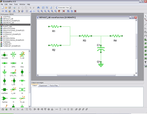
EcosimPro in schematic view, used for graphical models generation | |
| Stable release |
5.4.14
/ February 2015 |
|---|---|
| Preview release |
5.2.0
/ August 2013 |
| Operating system | Microsoft Windows |
| Website |
www |
EcosimPro is a simulation tool developed by Empresarios Agrupados A.I.E for modelling simple and complex physical processes that can be expressed in terms of Differential algebraic equations or Ordinary differential equations and Discrete event simulation.
The application runs on the various Microsoft Windows platforms and uses its own graphic environment for model design.
The modelling of physical components is based on the EcosimPro language (EL) which is very similar to other conventional Object-oriented programming[1] languages but is powerful enough to model continuous and discrete processes.
This tool employs a set of libraries containing various types of components (mechanical, electrical, pneumatic, hydraulic, etc.) that can be reused to model any type of system.
It is used within ESA for propulsion systems analysis[2] and is the recommended ESA analysis tool for ECLS systems.[3][4]
Origins
The EcosimPro Tool Project began in 1989 with funds from the European Space Agency (ESA) and with the goal of simulating environmental control and life support systems for manned spacecraft,[4] such as the Hermes shuttle. The multidisciplinary nature of this modelling tool led to its use in many other disciplines, including fluid mechanics, chemical processing, control, energy, propulsion and flight dynamics. These complex applications have demonstrated that EcosimPro is very robust and ready for use in many other fields.
The modelling language
Code examples
Differential equation
To familiarize yourself with the use of EcosimPro, first create a simple component to solve a differential equation. Although EcosimPro is designed to simulate complex systems, it can also be used independently of a physical system as if it were a pure equation solver. The example in this section illustrates this type of use. It solves the following differential equation to introduce a delay to variable x:

which is equivalent to

where x and y have a time dependence that will be defined in the experiment. Tau is datum provided given by the user; we will use a value of 0.6 seconds. This equation introduces a delay in the x variable with respect to y with value tau. To simulate this equation we will create an EcosimPro component with the equation in it.
The component to be simulated in EL is like thus:
COMPONENT equation_test
   DATA
      REAL tau = 0.6      "delay time (seconds)"
   DECLS
      REAL x, y
   CONTINUOUS
      y' = (x - y) / tau
END COMPONENT
Pendulum
One example of applied calculus could be the movement of a perfect pendulum (no friction taken into account). We would have the following data: the force of gravity ‘g’; the length of the pendulum ‘L’; and the pendulum’s mass ‘M’. As variables to be calculated we would have: the Cartesian position at each moment in time of the pendulum ‘x’ and ‘y’ and the tension on the wire of the pendulum ‘T’. The equations that define the model would be:
- Projecting the length of the cable on the Cartesian axes and applying Pythagoras’ theorem we get:

By decomposing force in Cartesians we get

and

To obtain the differential equations we can convert:

and

(note: is the first derivative of the position and equals the speed. is the second derivative of the position and equals the acceleration)


This example can be found in the DEFAULT_LIB library as “pendulum.el”:

COMPONENT pendulum   "Pendulum example"
   DATA
      REAL g = 9.806               "Gravity (m/s^2)"
      REAL L = 1.                  "Pendulum longitude (m)"
      REAL M = 1.                  "Pendulum mass (kg)"
   DECLS
      REAL x                       "Pendulum X position (m)"
      REAL y                       "Pendulum Y position (m)"
      REAL T                       "Pendulum wire tension force (N)"
   CONTINUOUS
      x**2 + y**2 = L**2
      M * x'' = - T * (x / L)
      M * y'' = - T * (y / L) - M * g
END COMPONENT
The last two equations respectively express the accelerations, x’’ and y’’, on the X and Y axes
Maths capabilities
- Symbolic handling of equations (e.g.: derivation, etc.)
- Robust solvers for non-linear and DAE systems: DASSL,[5] Newton-Raphson [6][7]
- Math wizards for:
- Defining boundary conditions
- Solving algebraic loops
- Reducing high-index DAE problems [8]
- Clever mathematical algorithms based on graph theory to minimize the number of unknown variables and equations
- Powerful discrete events handler to stop simulation when an event occurs
Applications
EcosimPro has been used in many fields and disciplines. The following paragraphs show several applications
- Control: This library provides components for the representation of control loops, including the typical P, PI and PID controllers, and signal processors, etc.
- Turbojet: Library for modelling turbine reactors. With components such as turbines, nozzles, compressors, burners, etc.
- ECLSS: A complete library of components has been developed to model complex environmental conditions for manned spacecraft[4]
- ESPSS: A standard set of libraries with components and functions for the simulation of launch vehicle propulsion systems and spacecraft propulsion systems.[2]
- Thermal: This library contains the components necessary to develop Lumped Parameter Thermal Models, i.e., diffusive thermal nodes, boundary thermal nodes, linear thermal conductors and radiative thermal conductors.
- Energy: In the field of Energy, EcosimPro has been used in different applications such as heat balances (Thermal_Balance), hydraulic systems (Pipe Networks Tool), molten carbonate and alkaline fuel cells, etc.
- Cryogenics: Simulation of large cryogenics systems, for instance, at CERN.[9]
- Others:
- Water treatment
- Waste treatment
- Agri-food Biotech processes
- Etc.
See also
References
- ↑ Bertrand Meyer (1997). Object Oriented Software Construction (2nd ed.). Prentice Hall. ISBN 0-13-629155-4.
- 1 2 Armin Isselhorst (July 2010). HM7B Simulation with ESPSS Tool on Ariane 5 ESC-A Upper Stage (PDF). 46th AIAA/ASME/SAE/ASEE Joint Propulsion Conference & Exhibit. AIAA. Retrieved May 6, 2011.
- ↑ "ESA: Thermal analysis software - EcosimPro". European Space Agency.
- 1 2 3 Daniele Laurini; Alan Thirkettle; Klaus Bockstahler (May 1999). "ESA: Supporting Life" (PDF). European Space Agency.
- ↑ Linda R. Petzold (1982). A Description of DASSL: A Differential/Algebraic System Solver SAND82-8637.
- ↑ P. Deuflhard (2004). Newton Methods for Nonlinear Problems. Affine Invariance and Adaptive Algorithms. Berlin: Springer. ISBN 3-540-21099-7.
- ↑ W. H. Press; B. P. Flannery; S. A. Teukolsky; W. T. Vetterling (1992). Numerical Recipes in C: The Art of Scientific Computing. Cambridge University Press. pp. sections 9.4 and 9.6 . ISBN 0-521-43108-5.
- ↑ C Pantelides (March 1988). "The Consistent Initialization of Differential-Algebraic Systems". SIAM J. Sci. Statist. Comput. 9: 213–231. doi:10.1137/0909014.
- ↑ B. Bradu; P. Gayet; S.I. Niculescu (2007). "A dynamic simulator for large scale cryogenic systems." (PDF). 6th EUROSIM Congress on Modelling and Simulation. Ljubljana, Slovenia. Retrieved May 6, 2011.