Factor analysis of mixed data
In statistics, factor analysis of mixed data (FAMD), or factorial analysis of mixed data, is the factorial method devoted to data tables in which a group of individuals is described both by quantitative and qualitative variables. It belongs to the exploratory methods developed by the French school called Analyse des données founded by Jean-Paul Benzécri.
The term mixed refers to the simultaneous presence, as active elements, of quantitative and qualitative variables. Roughly, we can say that FAMD works as a principal components analysis (PCA) for quantitative variables and as a multiple correspondence analysis (MCA) for qualitative variables.
Scope
When data include both types of variables but the active variables being homogeneous, PCA or MCA can be used.
Indeed, it is easy to include supplementary quantitative variables in MCA by the correlation coefficients between the variables and factors on individuals (a factor on individuals is the vector gathering the coordinates of individuals on a factorial axis); the representation obtained is a correlation circle (as in PCA).
Similarly, it is easy to include supplementary categorical variables in PCA.[1] For this, each category is represented by the center of gravity of the individuals who have it (as MCA).
Thus the presence of supplementary variables having a type different from the one of active variable does not pose any particular problem.
When the active variables are mixed, the usual practice is to perform discretization on the quantitative variables (e.g. usually in surveys the age is transformed in age classes). Data thus obtained can be processed by MCA.
This practice reaches its limits:
- When there are few individuals ( less than a hundred to fix ideas ) in which case the MCA is unstable ;
- When there are few qualitative variables with respect to quantitative variables (one can be reluctant to discretize twenty quantitative variables to take into account a single qualitative variable).
Criterion
The data include  quantitative variables
  and
and  qualitative variables
  .
.
 is a quantitative variable. We note:
-
 the correlation coefficient between variables
  and ;
and ; -
 the squared correlation ratio between variables and
  .
.
In the PCA of , we look for the function on  (a function on assigns a value to each individual, it is the case for initial variables and principal components) the most correlated to all variables in the following sense:
-
 maximum.
In MCA of Q, we look for the function on more related to all variables in the following sense:
-
 maximum.
In FAMD  , we look for the function on the more related to all
  variables in the following sense:
-
 maximum.
In this criterion, both types of variables play the same role. The contribution of each variable in this criterion is bounded by 1.
Plots
The representation of individuals is made directly from factors .
The representation of quantitative variables is constructed as in PCA (correlation circle).
The representation of the categories of qualitative variables is as in MCA : a category is at the centroid of the individuals who possess it. Note that we take the exact centroid and not, as is customary in MCA, the centroid up to a coefficient dependent on the axis (in MCA this coefficient is equal to the inverse of the square root of the eigenvalue; it would be inadequate in FAMD).
The representation of variables is called relationship square. The coordinate of qualitative variable  along axis
  is equal to squared correlation ratio between the variable and the factor of rank (denoted
  ). The coordinates of quantitative variable along axis is equal to the squared correlation coefficient between the variable and the factor of rank (denoted
  ).
).
Aids to interpretation
The relationship indicators between the initial variables are combined in a so-called relationship matrix that contains, at the intersection of row  and column
  :
:
- If the variables and are quantitative, the squared correlation coefficient between the variables and ;
- If the variable is qualitative and the variable is quantitative, the squared correlation ratio between and ;
- If the variables and are qualitative, the indicator
 between the variables and .
Example
A very small data set (Table 1) illustrates the operation and outputs of the FAMD . Six individuals are described by three quantitative variables and three qualitatives variables. Data were analyzed using the R package function FAMD FactoMineR .
|
|


In the relationship matrix, the coefficients are equal to  (quantitative variables), (qualitative variables) or
  (one variable of each type).
The matrix shows an entanglement of the relationships between the two types of variables.
The representation of individuals (Figure 1) clearly shows three groups of individuals. The first axis opposes individuals 1 and 2 to all others. The second axis opposes individuals 3 and 4 to individuals 5 and 6.
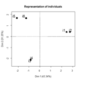 Figure1. FAMD. Test example. Representation of individuals. |
 Figure2. FAMD. Test example. Relationship square. |
 Figure3. FAMD. Test example. Correlation circle. |
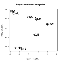 Figure4. FAMD. Test example. Representation of the categories of qualitative variables. |
The representation of variables (relationship square, Figure 2) shows that the first axis ( ) is closely linked to variables
  ,
,  and
and  . The correlation circle (Figure 3) specifies the sign of the correlation between , and ; the representation of the categories (Figure 4) clarifies the nature of the relationship between and . Finally individuals 1 and 2, individualized by the first axis, are characterized by high values of and and by the categories of as well.
This example illustrates how the FAMD simultaneously analyses of quantitative and qualitative variables. Thus, it shows, in this example, a first dimension based on the two types of variables.
History
The FAMD 's original work is due to Brigitte Escofier[2] and Gilbert Saporta.[3] This work was resumed in 2002 by Jérôme Pagès.[4] The most complete presentation of FAMD in English is included in a book of Jérôme Pagès.[5]
References
- ↑ Escofier Brigitte & Pagès Jérôme (2008). Analyses factorielles simples et multiples. Dunod. Paris. 318 p. p. 27 et seq.
- ↑ Escofier Brigitte (1979). Traitement simultané de variables quantitatives et qualitatives en analyse factorielle. Les cahiers de l’analyse des données, 4, 2, 137–146. http://archive.numdam.org/ARCHIVE/CAD/CAD_1979__4_2/CAD_1979__4_2_137_0/CAD_1979__4_2_137_0.pdf
- ↑ Saporta Gilbert (1990). Simultaneous analysis of qualitative and quantitative data. Atti della XXXV riunione scientifica ; società italiana di Statistica, 63–72 . http://cedric.cnam.fr/~saporta/SAQQD.pdf
- ↑ Pagès Jérôme (2002). Analyse factorielle de données mixtes. Revue de Statistique appliquée, 52, 4, 93–111 http://archive.numdam.org/ARCHIVE/RSA/RSA_2004__52_4/RSA_2004__52_4_93_0/RSA_2004__52_4_93_0.pdf
- ↑ Pagès Jérôme (2014). Multiple Factor Analysis by Example Using R. Chapman & Hall/CRC The R Series London 272 p