Knapsack problem

Example of a one-dimensional (constraint) knapsack problem: which boxes should be chosen to maximize the amount of money while still keeping the overall weight under or equal to 15 kg? A multiple constrained problem could consider both the weight and volume of the boxes.
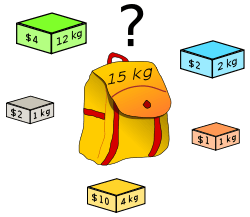
(Solution: if any number of each box is available, then three yellow boxes and three grey boxes; if only the shown boxes are available, then all but the green box.)

The knapsack problem or rucksack problem is a problem in combinatorial optimization: Given a set of items, each with a weight and a value, determine the number of each item to include in a collection so that the total weight is less than or equal to a given limit and the total value is as large as possible. It derives its name from the problem faced by someone who is constrained by a fixed-size knapsack and must fill it with the most valuable items.

The problem often arises in resource allocation where there are financial constraints and is studied in fields such as combinatorics, computer science, complexity theory, cryptography, applied mathematics, and daily fantasy sports.

The knapsack problem has been studied for more than a century, with early works dating as far back as 1897.^[1] The name "knapsack problem" dates back to the early works of mathematician Tobias Dantzig (1884–1956),^[2] and refers to the commonplace problem of packing your most valuable or useful items without overloading your luggage.

Applications

A 1998 study of the Stony Brook University Algorithm Repository showed that, out of 75 algorithmic problems, the knapsack problem was the 18th most popular and the 4th most needed after kd-trees, suffix trees, and the bin packing problem.^[3]

Knapsack problems appear in real-world decision-making processes in a wide variety of fields, such as finding the least wasteful way to cut raw materials,^[4] selection of investments and portfolios,^[5] selection of assets for asset-backed securitization,^[6] and generating keys for the Merkle–Hellman^[7] and other knapsack cryptosystems.

One early application of knapsack algorithms was in the construction and scoring of tests in which the test-takers have a choice as to which questions they answer. For small examples it is a fairly simple process to provide the test-takers with such a choice. For example, if an exam contains 12 questions each worth 10 points, the test-taker need only answer 10 questions to achieve a maximum possible score of 100 points. However, on tests with a heterogeneous distribution of point values—i.e. different questions are worth different point values— it is more difficult to provide choices. Feuerman and Weiss proposed a system in which students are given a heterogeneous test with a total of 125 possible points. The students are asked to answer all of the questions to the best of their abilities. Of the possible subsets of problems whose total point values add up to 100, a knapsack algorithm would determine which subset gives each student the highest possible score.^[8]

Definition

The most common problem being solved is the 0-1 knapsack problem, which restricts the number x_i of copies of each kind of item to zero or one. Given a set of n items numbered from 1 up to n, each with a weight w_i and a value v_i, along with a maximum weight capacity W,

maximize $\sum _{i=1}^{n}v_{i}x_{i}$

subject to $\sum _{i=1}^{n}w_{i}x_{i}\leq W$ and $x_{i}\in \{0,1\}$.

Here x_i represents the number of instances of item i to include in the knapsack. Informally, the problem is to maximize the sum of the values of the items in the knapsack so that the sum of the weights is less than or equal to the knapsack's capacity.

The bounded knapsack problem (BKP) removes the restriction that there is only one of each item, but restricts the number $x_{i}$ of copies of each kind of item to a maximum non-negative integer value $c$:

maximize $\sum _{i=1}^{n}v_{i}x_{i}$

subject to $\sum _{i=1}^{n}w_{i}x_{i}\leq W$ and ${\displaystyle 0\leq x_{i}\leq c}$

The unbounded knapsack problem (UKP) places no upper bound on the number of copies of each kind of item and can be formulated as above except for that the only restriction on $x_{i}$ is that it is a non-negative integer.

maximize $\sum _{i=1}^{n}v_{i}x_{i}$

subject to $\sum _{i=1}^{n}w_{i}x_{i}\leq W$ and $x_{i}\geq 0$

One example of the unbounded knapsack problem is given using the figure shown at the beginning of this article and the text "if any number of each box is available" in the caption of that figure.

Computational complexity

The knapsack problem is interesting from the perspective of computer science for many reasons:

• The decision problem form of the knapsack problem (Can a value of at least V be achieved without exceeding the weight W?) is NP-complete, thus there is no known algorithm both correct and fast (polynomial-time) on all cases.
• While the decision problem is NP-complete, the optimization problem is NP-hard, its resolution is at least as difficult as the decision problem, and there is no known polynomial algorithm which can tell, given a solution, whether it is optimal (which would mean that there is no solution with a larger V, thus solving the NP-complete decision problem).
• There is a pseudo-polynomial time algorithm using dynamic programming.
• There is a fully polynomial-time approximation scheme, which uses the pseudo-polynomial time algorithm as a subroutine, described below.
• Many cases that arise in practice, and "random instances" from some distributions, can nonetheless be solved exactly.

There is a link between the "decision" and "optimization" problems in that if there exists a polynomial algorithm that solves the "decision" problem, then one can find the maximum value for the optimization problem in polynomial time by applying this algorithm iteratively while increasing the value of k . On the other hand, if an algorithm finds the optimal value of optimization problem in polynomial time, then the decision problem can be solved in polynomial time by comparing the value of the solution output by this algorithm with the value of k . Thus, both versions of the problem are of similar difficulty.

One theme in research literature is to identify what the "hard" instances of the knapsack problem look like,^[9][10] or viewed another way, to identify what properties of instances in practice might make them more amenable than their worst-case NP-complete behaviour suggests.^[11] The goal in finding these "hard" instances is for their use in public key cryptography systems, such as the Merkle-Hellman knapsack cryptosystem.

Solving

Several algorithms are available to solve knapsack problems, based on dynamic programming approach,^[12] branch and bound approach^[13] or hybridizations of both approaches.^{[11][14][15][16]}

Dynamic programming in-advance algorithm

Unbounded knapsack problem

If all weights ($w_{1},\ldots ,w_{n}$) are nonnegative integers, the knapsack problem can be solved in pseudo-polynomial time using dynamic programming. The following describes a dynamic programming solution for the unbounded knapsack problem.

To simplify things, assume all weights are strictly positive ($w_{i}>0$). We wish to maximize total value subject to the constraint that total weight is less than or equal to $W$. Then for each $w\leq W$, define $m[w]$ to be the maximum value that can be attained with total weight less than or equal to $w$. Then, $m[W]$ is the solution to the problem.

Observe that $m[w]$ has the following properties:

• $m[0]=0\,\!$ (the sum of zero items, i.e., the summation of the empty set)
• $m[w]=\max _{w_{i}\leq w}(v_{i}+m[w-w_{i}])$

where $v_{i}$ is the value of the i-th kind of item.

(To formulate the equation above, the idea used is that the solution for a knapsack is the same as the value of one correct item plus the solution for a knapsack with smaller capacity, specifically one with the capacity reduced by the weight of that chosen item.)

Here the maximum of the empty set is taken to be zero. Tabulating the results from $m[0]$ up through $m[W]$ gives the solution. Since the calculation of each $m[w]$ involves examining $n$ items, and there are $W$ values of $m[w]$ to calculate, the running time of the dynamic programming solution is $O(nW)$. Dividing $w_{1},\,w_{2},\,\ldots ,\,w_{n},\,W$ by their greatest common divisor is a way to improve the running time.

The $O(nW)$ complexity does not contradict the fact that the knapsack problem is NP-complete, since $W$, unlike $n$, is not polynomial in the length of the input to the problem. The length of the $W$ input to the problem is proportional to the number of bits in $W$, $\log W$, not to $W$ itself.

0/1 knapsack problem

A similar dynamic programming solution for the 0/1 knapsack problem also runs in pseudo-polynomial time. Assume $w_{1},\,w_{2},\,\ldots ,\,w_{n},\,W$ are strictly positive integers. Define $m[i,w]$ to be the maximum value that can be attained with weight less than or equal to $w$ using items up to $i$ (first $i$ items).

We can define $m[i,w]$ recursively as follows:

• $m[0,\,w]=0$
• $m[i,\,w]=m[i-1,\,w]$ if $w_{i}>w\,\!$ (the new item is more than the current weight limit)
• $m[i,\,w]=\max(m[i-1,\,w],\,m[i-1,w-w_{i}]+v_{i})$ if $w_{i}\leqslant w$.

The solution can then be found by calculating $m[n,W]$. To do this efficiently we can use a table to store previous computations.

The following is pseudo code for the dynamic program:

 1 // Input:
 2 // Values (stored in array v)
 3 // Weights (stored in array w)
 4 // Number of distinct items (n)
 5 // Knapsack capacity (W)
 6 
 7 for j from 0 to W do:
 8     m[0, j] := 0
 9 
10 for i from 1 to n do:
11     for j from 0 to W do:
12         if w[i] > j then:
13             m[i, j] := m[i-1, j]
14         else:
15             m[i, j] := max(m[i-1, j], m[i-1, j-w[i]] + v[i])

This solution will therefore run in $O(nW)$ time and $O(nW)$ space. Additionally, if we use only a 1-dimensional array $m[w]$ to store the current optimal values and pass over this array $i+1$ times, rewriting from $m[W]$ to $m[1]$ every time, we get the same result for only $O(W)$ space.

Meet-in-the-middle

Another algorithm for 0-1 knapsack, discovered in 1974 ^[17] and sometimes called "meet-in-the-middle" due to parallels to a similarly named algorithm in cryptography, is exponential in the number of different items but may be preferable to the DP algorithm when $W$ is large compared to n. In particular, if the $w_{i}$ are nonnegative but not integers, we could still use the dynamic programming algorithm by scaling and rounding (i.e. using fixed-point arithmetic), but if the problem requires $d$ fractional digits of precision to arrive at the correct answer, $W$ will need to be scaled by $10^{d}$, and the DP algorithm will require ${\displaystyle O(W10^{d})}$ space and ${\displaystyle O(nW10^{d})}$ time.

Meet-in-the-middle algorithm

  input: 
    a set of items with weights and values
  output: 
    the greatest combined value of a subset
  partition the set {1...n} into two sets A and B of approximately equal size
  compute the weights and values of all subsets of each set
  for each subset of A
    find the subset of B of greatest value such that the combined weight is less than W
  keep track of the greatest combined value seen so far

The algorithm takes $O(2^{n/2})$ space, and efficient implementations of step 3 (for instance, sorting the subsets of B by weight, discarding subsets of B which weigh more than other subsets of B of greater or equal value, and using binary search to find the best match) result in a runtime of ${\displaystyle O(n2^{n/2})}$. As with the meet in the middle attack in cryptography, this improves on the $O(n*2^{n})$ runtime of a naive brute force approach (examining all subsets of {1...n}), at the cost of using exponential rather than constant space (see also baby-step giant-step).

Approximation algorithms

As for most NP-complete problems, it may be enough to find workable solutions even if they are not optimal. Preferably, however, the approximation comes with a guarantee on the difference between the value of the solution found and the value of the optimal solution.

As with many useful but computationally complex algorithms, there has been substantial research on creating and analyzing algorithms that approximate a solution. The knapsack problem, though NP-Hard, is one of a collection of algorithms that can still be approximated to any specified degree. This means that the problem has a polynomial time approximation scheme. To be exact, the knapsack problem has a fully polynomial time approximation scheme (FPTAS).^[18]

Greedy approximation algorithm

George Dantzig proposed a greedy approximation algorithm to solve the unbounded knapsack problem.^[19] His version sorts the items in decreasing order of value per unit of weight, $v_{i}/w_{i}$. It then proceeds to insert them into the sack, starting with as many copies as possible of the first kind of item until there is no longer space in the sack for more. Provided that there is an unlimited supply of each kind of item, if $m$ is the maximum value of items that fit into the sack, then the greedy algorithm is guaranteed to achieve at least a value of $m/2$. However, for the bounded problem, where the supply of each kind of item is limited, the algorithm may be far from optimal.

Fully polynomial time approximation scheme

The fully polynomial time approximation scheme (FPTAS) for the knapsack problem takes advantage of the fact that the reason the problem has no known polynomial time solutions is because the profits associated with the items are not restricted. If one rounds off some of the least significant digits of the profit values then they will be bounded by a polynomial and 1/ε where ε is a bound on the correctness of the solution. This restriction then means that an algorithm can find a solution in polynomial time that is correct within a factor of (1-ε) of the optimal solution.^[18]

An Algorithm for FPTAS

 input: 
   ε ∈ [0,1]
   a list A of n items, specified by their values, $v_{i}$, and weights
 output:
   S' the FPTAS solution

 P := max $\{v_{i}\mid 1\leq i\leq n\}$  // the highest item value
 K := ε ${\displaystyle {\frac {P}{n}}}$
 for i from 1 to n do
    $v'_{i}$ := ${\displaystyle \left\lfloor {\frac {v_{i}}{K}}\right\rfloor }$
 end for
 return the solution, S', using the $v'_{i}$ values in the dynamic program outlined above

Theorem: The set $S'$ computed by the algorithm above satisfies $\mathrm {profit} (S')\geq (1-\varepsilon )\cdot \mathrm {profit} (S^{*})$, where $S^{*}$ is an optimal solution.

Dominance relations

Solving the unbounded knapsack problem can be made easier by throwing away items which will never be needed. For a given item i, suppose we could find a set of items J such that their total weight is less than the weight of i, and their total value is greater than the value of i. Then i cannot appear in the optimal solution, because we could always improve any potential solution containing i by replacing i with the set J. Therefore, we can disregard the i-th item altogether. In such cases, J is said to dominate i. (Note that this does not apply to bounded knapsack problems, since we may have already used up the items in J.)

Finding dominance relations allows us to significantly reduce the size of the search space. There are several different types of dominance relations,^[11] which all satisfy an inequality of the form:

$\qquad \sum _{j\in J}w_{j}\,x_{j}\ \leq \alpha \,w_{i}$, and ${\displaystyle \sum _{j\in J}v_{j}\,x_{j}\ \geq \alpha \,v_{i}\,}$ for some $x\in Z_{+}^{n}$

where ${\displaystyle \alpha \in Z_{+}\,,J\subsetneq N}$ and $i\not \in J$. The vector $x$ denotes the number of copies of each member of J.

Collective dominance

The i-th item is collectively dominated by J, written as $i\ll J$, if the total weight of some combination of items in J is less than w_i and their total value is greater than v_i. Formally, ${\displaystyle \sum _{j\in J}w_{j}\,x_{j}\ \leq w_{i}}$ and ${\displaystyle \sum _{j\in J}v_{j}\,x_{j}\ \geq v_{i}}$ for some $x\in Z_{+}^{n}$, i.e. $\alpha =1$. Verifying this dominance is computationally hard, so it can only be used with a dynamic programming approach. In fact, this is equivalent to solving a smaller knapsack decision problem where ${\displaystyle V=v_{i}}$, ${\displaystyle W=w_{i}}$, and the items are restricted to J.

Threshold dominance

The i-th item is threshold dominated by J, written as $i\prec \prec J$, if some number of copies of $i$ are dominated by J. Formally, ${\displaystyle \sum _{j\in J}w_{j}\,x_{j}\ \leq \alpha \,w_{i}}$, and ${\displaystyle \sum _{j\in J}v_{j}\,x_{j}\ \geq \alpha \,v_{i}\,}$ for some $x\in Z_{+}^{n}$ and $\alpha \geq 1$. This is a generalization of collective dominance, first introduced in^[12] and used in the EDUK algorithm. The smallest such $\alpha$ defines the threshold of the item $i$, written $t_{i}=(\alpha -1)w_{i}$. In this case, the optimal solution could contain at most $\alpha -1$ copies of $i$.

Multiple dominance

The i-th item is multiply dominated by a single item $j$, written as $i\ll _{m}j$, if $i$ is dominated by some number of copies of $j$. Formally, ${\displaystyle w_{j}\,x_{j}\ \leq w_{i}}$, and ${\displaystyle v_{j}\,x_{j}\ \geq v_{i}}$ for some $x_{j}\in Z_{+}$ i.e. $J=\{j\},\alpha =1,x_{j}=\lfloor {\frac {w_{i}}{w_{j}}}\rfloor$. This dominance could be efficiently used during preprocessing because it can be detected relatively easily.

Modular dominance

Let b be the best item, i.e. ${\frac {v_{b}}{w_{b}}}\geq {\frac {v_{i}}{w_{i}}}\,$ for all $i$. This is the item with the greatest density of value. The i-th item is modularly dominated by a single item $j$, written as $i\ll _{\equiv }j$, if $i$ is dominated by $j$ plus several copies of b. Formally, $w_{j}+tw_{b}\leq w_{i}$, and $v_{j}+tv_{b}\geq v_{i}$ i.e. $J=\{b,j\},\alpha =1,x_{b}=t,x_{j}=1$.

Variations

There are many variations of the knapsack problem that have arisen from the vast number of applications of the basic problem. The main variations occur by changing the number of some problem parameter such as the number of items, number of objectives, or even the number of knapsacks.

Multi-objective knapsack problem

This variation changes the goal of the individual filling the knapsack. Instead of one objective, such as maximizing the monetary profit, the objective could have several dimensions. For example, there could be environmental or social concerns as well as economic goals. Problems frequently addressed include portfolio and transportation logistics optimizations.^[20][21]

As a concrete example, suppose you ran a cruise ship. You have to decide how many famous comedians to hire. This boat can handle no more than one ton of passengers and the entertainers must weigh less than 1000 lbs. Each comedian has a weight, brings in business based on their popularity and asks for a specific salary. In this example you have multiple objectives. You want, of course, to maximize the popularity of your entertainers while minimizing their salaries. Also, you want to have as many entertainers as possible.

Multi-dimensional knapsack problem

In this variation, the weight of knapsack item $i$ is given by a D-dimensional vector ${\overline {w_{i}}}=(w_{i1},\ldots ,w_{iD})$ and the knapsack has a D-dimensional capacity vector $(W_{1},\ldots ,W_{D})$. The target is to maximize the sum of the values of the items in the knapsack so that the sum of weights in each dimension $d$ does not exceed $W_{d}$.

Multi-dimensional knapsack is computationally harder than knapsack; even for $D=2$, the problem does not have EPTAS unless P$=$NP.^[22] However, the algorithm in ^[23] is shown to solve sparse instances efficiently. An instance of multi-dimensional knapsack is sparse if there is a set $J=\{1,2,\ldots ,m\}$ for $m<D$ such that for every knapsack item $i$, $\exists z>m$ such that $\forall j\in J\cup \{z\},\ w_{ij}\geq 0$ and $\forall y\notin J\cup \{z\},w_{iy}=0$. Such instances occur, for example, when scheduling packets in a wireless network with relay nodes.^[23] The algorithm from ^[23] also solves sparse instances of the multiple choice variant, multiple-choice multi-dimensional knapsack.

The IHS (Increasing Height Shelf) algorithm is optimal for 2D knapsack (packing squares into a two-dimensional unit size square): when there are at most five square in an optimal packing.^[24]

Multiple knapsack problem

This variation is similar to the Bin Packing Problem. It differs from the Bin Packing Problem in that a subset of items can be selected, whereas, in the Bin Packing Problem, all items have to be packed to certain bins. The concept is that there are multiple knapsacks. This may seem like a trivial change, but it is not equivalent to adding to the capacity of the initial knapsack. This variation is used in many loading and scheduling problems in Operations Research and has a PTAS^[25]

Quadratic knapsack problem

As described by Wu et al.:

The quadratic knapsack problem (QKP) maximizes a quadratic objective function subject to a binary and linear capacity constraint.^[26]

The quadratic knapsack problem was discussed under that title by Gallo, Hammer, and Simeone in 1980.^[27] However, Gallo and Simeone^[28] attribute the first treatment of the problem to Witzgall^[29] in 1975.

Subset-sum problem

The subset sum problem is a special case of the decision and 0-1 problems where each kind of item, the weight equals the value: $w_{i}=v_{i}$. In the field of cryptography, the term knapsack problem is often used to refer specifically to the subset sum problem and is commonly known as one of Karp's 21 NP-complete problems.^[30]

The generalization of subset sum problem is called multiple subset-sum problem, in which multiple bins exist with the same capacity. It has been shown that the generalization does not have an FPTAS.^[31]

Software

Name	License	Brief info
PAAL	BOOST LICENSE	Approximation algorithms library containing generic and efficient implementations of various knapsack algorithms including: dynamic algorithm, greedy (2-approximation) and FPTAS. The above algorithms are implemented for both 0/1 and unbounded versions of the problem.[32]
OpenOpt	BSD	Free Python language framework that can use either free or commercial MILP and other solvers to solve knapsack problems, possibly constrained, nonlinear and multiobjective.[33][34]
adagio	GPL	R's CRAN package adagio provides methods and algorithms for discrete optimization and (evolutionary) global optimization.[35]
Algorithm::Knapsack	Perl 5	Algorithm::Knapsack is a simple Perl module that solves 0/1 versions of the knapsack problem.[36]
FORTRAN Codes	Free for non-commercial use	Codes.zip is a library of FORTRAN implementations of exact and approximation algorithms for a variety of single and multiple knapsack problems. [37]

Popular culture

• Neal Stephenson provides an example of the knapsack problem in chapter 70 of his novel, Cryptonomicon, to distribute family heirlooms.
• The knapsack problem occurs commonly in role-playing games, both digital and paper-based (prominent examples include The Elder Scrolls series and the Dungeons and Dragons game, respectively), where the player character is constrained by their encumbrance threshold when carrying items and treasure, which regularly forces the player to evaluate the items' value-to-weight ratio in order to bring only the most value-dense items to a merchant.

See also

• Change-making problem
• Combinatorial auction
• Combinatorial optimization
• Continuous knapsack problem
• Cutting stock problem
• List of knapsack problems
• Packing problem

Notes

1. Mathews, G. B. (25 June 1897). "On the partition of numbers" (PDF). Proceedings of the London Mathematical Society. 28: 486–490. doi:10.1112/plms/s1-28.1.486.
2. Dantzig, Tobias. Numbers: The Language of Science, 1930.
3. Skiena, S. S. (September 1999). "Who is Interested in Algorithms and Why? Lessons from the Stony Brook Algorithm Repository". AGM SIGACT News. 30 (3): 65–74. doi:10.1145/333623.333627. ISSN 0163-5700.
4. Kellerer, Pferschy, and Pisinger 2004, p. 449
5. Kellerer, Pferschy, and Pisinger 2004, p. 461
6. Kellerer, Pferschy, and Pisinger 2004, p. 465
7. Kellerer, Pferschy, and Pisinger 2004, p. 472
8. Feuerman, Martin; Weiss, Harvey (April 1973). "A Mathematical Programming Model for Test Construction and Scoring". Management Science. 19 (8): 961–966. doi:10.1287/mnsc.19.8.961. JSTOR 2629127.
9. Pisinger, D. 2003. Where are the hard knapsack problems? Technical Report 2003/08, Department of Computer Science, University of Copenhagen, Copenhagen, Denmark.
10. Caccetta, L.; Kulanoot, A. (2001). "Computational Aspects of Hard Knapsack Problems". Nonlinear Analysis. 47: 5547–5558. doi:10.1016/s0362-546x(01)00658-7.
11. Poirriez, Vincent; Yanev, Nicola; Andonov, Rumen (2009). "A hybrid algorithm for the unbounded knapsack problem". Discrete Optimization. 6 (1): 110–124. doi:10.1016/j.disopt.2008.09.004. ISSN 1572-5286.
12. Andonov, Rumen; Poirriez, Vincent; Rajopadhye, Sanjay (2000). "Unbounded Knapsack Problem : dynamic programming revisited". European Journal of Operational Research. 123 (2): 168–181. doi:10.1016/S0377-2217(99)00265-9.
13. S. Martello, P. Toth, Knapsack Problems: Algorithms and Computer Implementations, John Wiley and Sons, 1990
14. S. Martello, D. Pisinger, P. Toth, Dynamic programming and strong bounds for the 0-1 knapsack problem, Manag. Sci., 45:414–424, 1999.
15. Plateau, G.; Elkihel, M. (1985). "A hybrid algorithm for the 0-1 knapsack problem". Methods of Oper. Res. 49: 277–293.
16. Martello, S.; Toth, P. "A mixture of dynamic programming and branch-and-bound for the subset-sum problem". Manag. Sci. 30: 765–771. doi:10.1287/mnsc.30.6.765.
17. Horowitz, Ellis; Sahni, Sartaj (1974), "Computing partitions with applications to the knapsack problem", Journal of the Association for Computing Machinery, 21: 277–292, doi:10.1145/321812.321823, MR 0354006
18. Vazirani, Vijay. Approximation Algorithms. Springer-Verlag Berlin Heidelberg, 2003.
19. Dantzig, George B. (1957). "Discrete-Variable Extremum Problems". Operations Research. 5 (2): 266–288. doi:10.1287/opre.5.2.266.
20. Chang, T. J., et al. Heuristics for Cardinality Constrained Portfolio Optimization. Technical Report, London SW7 2AZ, England: The Management School, Imperial College, May 1998
21. Chang, C. S., et al. "Genetic Algorithm Based Bicriterion Optimization for Traction Substations in DC Railway System." In Fogel [102], 11-16.
22. Kulik, A.; Shachnai, H. (2010). "There is no EPTAS for two dimensional knapsack". Inf. Process. Lett. 110 (16): 707–710. doi:10.1016/j.ipl.2010.05.031.
23. Cohen, R. and Grebla, G. 2014. "Multi-Dimensional OFDMA Scheduling in a Wireless Network with Relay Nodes". in Proc. IEEE INFOCOM’14, 2427–2435.
24. Yan Lan, György Dósa, Xin Han, Chenyang Zhou, Attila Benkő : 2D knapsack: Packing squares, Theoretical Computer Science Vol. 508, pp. 35–40.
25. Chandra Chekuri and Sanjeev Khanna. 2000. A PTAS for the multiple knapsack problem. In Proceedings of the eleventh annual ACM-SIAM symposium on Discrete algorithms (SODA '00). Society for Industrial and Applied Mathematics, Philadelphia, PA, USA, 213-222.
26. Wu, Z. Y.; Yang, Y. J.; Bai, F. S.; Mammadov, M. (2011). "Global Optimality Conditions and Optimization Methods for Quadratic Knapsack Problems". J Optim Theory Appl. 151: 241–259. doi:10.1007/s10957-011-9885-4.
27. Gallo, G.; Hammer, P. L.; Simeone, B. (1980). "Quadratic knapsack problems". Mathematical Programming Studies. 12: 132–149. doi:10.1007/BFb0120892.
28. Gallo, G.; Simeone, B. (1988). "On the Supermodular Knapsack Problem". Mathematical Programming Studies. North-Holland. 45: 295–309. doi:10.1007/bf01589108.
29. Witzgall, C. (1975). Mathematical methods of site selection for Electronic Message Systems (EMS). NBS Internal report.
30. Richard M. Karp (1972). "Reducibility Among Combinatorial Problems". In R. E. Miller and J. W. Thatcher (editors). Complexity of Computer Computations. New York: Plenum. pp. 85–103
31. Caprara, Alberto; Kellerer, Hans; Pferschy, Ulrich (2000). "The Multiple Subset Sum Problem". SIAM J. on Optimization. 11 (2): 308–319. doi:10.1137/S1052623498348481.
32. "PAAL". paal.mimuw.edu.pl. Retrieved 2014-10-03.
33. "KSP". OpenOpt. Retrieved 2014-04-06.
34. "Problems". OpenOpt. Retrieved 2014-04-06.
35. "CRAN - Package adagio". Cran.r-project.org. 2013-09-28. Retrieved 2014-04-06.
36. "MetaCPAN - Algorithm::Knapsack". Alexander Anderson. Retrieved 2015-07-09.
37. "Knapsack problems: Algorithms and computer implementations".

References

• Garey, Michael R.; David S. Johnson (1979). Computers and Intractability: A Guide to the Theory of NP-Completeness. W.H. Freeman. ISBN 0-7167-1045-5. A6: MP9, pg.247.
• Kellerer, Hans; Pferschy, Ulrich; Pisinger, David (2004). Knapsack Problems. Springer. doi:10.1007/978-3-540-24777-7. ISBN 3-540-40286-1. MR 2161720.
• Martello, Silvano; Toth, Paolo (1990). Knapsack problems: Algorithms and computer implementations. Wiley-Interscience. ISBN 0-471-92420-2. MR 1086874.

External links

• Free download of the book "Knapsack problems: Algorithms and computer implementations", by Silvano Martello and Paolo Toth
• Lecture slides on the knapsack problem
• PYAsUKP: Yet Another solver for the Unbounded Knapsack Problem, with code taking advantage of the dominance relations in an hybrid algorithm, benchmarks and downloadable copies of some papers.
• Home page of David Pisinger with downloadable copies of some papers on the publication list (including "Where are the hard knapsack problems?")
• Knapsack Problem solutions in many languages at Rosetta Code
• Dynamic Programming algorithm to 0/1 Knapsack problem
• Knapsack Problem solver (online)
• Interactive JavaScript branch-and-bound solver
• Solving 0-1-KNAPSACK with Genetic Algorithms in Ruby
• Codes for Quadratic Knapsack Problem