Lagrange polynomial

In numerical analysis, Lagrange polynomials are used for polynomial interpolation. For a given set of distinct points and numbers , the Lagrange polynomial is the polynomial of the least degree that at each point assumes the corresponding value (i.e. the functions coincide at each point). The interpolating polynomial of the least degree is unique, however, and it is therefore more appropriate to speak of "the Lagrange form" of that unique polynomial rather than "the Lagrange interpolation polynomial", since the same polynomial can be arrived at through multiple methods. Although named after Joseph Louis Lagrange, who published it in 1795, it was first discovered in 1779 by Edward Waring and it is also an easy consequence of a formula published in 1783 by Leonhard Euler.[1]


Lagrange interpolation is susceptible to Runge's phenomenon, and the fact that changing the interpolation points requires recalculating the entire interpolant can make Newton polynomials easier to use. Lagrange polynomials are used in the Newton–Cotes method of numerical integration and in Shamir's secret sharing scheme in cryptography.
Definition
Given a set of k + 1 data points

where no two are the same, the interpolation polynomial in the Lagrange form is a linear combination

of Lagrange basis polynomials

where . Note how, given the initial assumption that no two are the same, , so this expression is always well-defined. The reason pairs with are not allowed is that no interpolation function such that would exist; a function can only get one value for each argument . On the other hand, if also , then those two points would actually be one single point.


For all , includes the term in the numerator, so the whole product will be zero at :


On the other hand,

In other words, all basis polynomials are zero at , except , for which it holds that , because it lacks the term.


It follows that , so at each point , , showing that interpolates the function exactly.


Proof
The function L(x) being sought is a polynomial in of the least degree that interpolates the given data set; that is, assumes value at the corresponding for all data points :


Observe that:
- In there are k factors in the product and each factor contains one x, so L(x) (which is a sum of these k-degree polynomials) must also be a k-degree polynomial.

We consider what happens when this product is expanded. Because the product skips , if then all terms are (except where , but that case is impossible, as pointed out in the definition section—in that term, , and since , , contrary to ). Also if then since does not preclude it, one term in the product will be for , i.e. , zeroing the entire product. So


where is the Kronecker delta. So:


Thus the function L(x) is a polynomial with degree at most k and where .

Additionally, the interpolating polynomial is unique, as shown by the unisolvence theorem at the polynomial interpolation article.
Main idea
Solving an interpolation problem leads to a problem in linear algebra amounting to inversion of a matrix. Using a standard monomial basis for our interpolation polynomial L(x) =∑j=0k x j mj, we must invert the Vandermonde matrix (xi ) j to solve L(xi) = yi for the coefficients mj of L(x). By choosing a better basis, the Lagrange basis, L(x) = ∑j=0k lj(x) yj, we merely get the identity matrix, δij, which is its own inverse: the Lagrange basis automatically inverts the analog of the Vandermonde matrix.
This construction is analogous to the Chinese Remainder Theorem. Instead of checking for remainders of integers modulo prime numbers, we are checking for remainders of polynomials when divided by linears.
Examples
Example 1
We wish to interpolate ƒ(x) = x2 over the range 1 ≤ x ≤ 3, given these three points:

The interpolating polynomial is:
![{\begin{aligned}L(x)&={1}\cdot {x-2 \over 1-2}\cdot {x-3 \over 1-3}+{4}\cdot {x-1 \over 2-1}\cdot {x-3 \over 2-3}+{9}\cdot {x-1 \over 3-1}\cdot {x-2 \over 3-2}\\[10pt]&=x^{2}.\end{aligned}}](../I/m/274ccc9dab43ec4880e953e43ebcd5a8470cf12a.svg)
Example 2
We wish to interpolate ƒ(x) = x3 over the range 1 ≤ x ≤ 3, given these three points:


The interpolating polynomial is:
![{\begin{aligned}L(x)&={1}\cdot {x-2 \over 1-2}\cdot {x-3 \over 1-3}+{8}\cdot {x-1 \over 2-1}\cdot {x-3 \over 2-3}+{27}\cdot {x-1 \over 3-1}\cdot {x-2 \over 3-2}\\[8pt]&=6x^{2}-11x+6.\end{aligned}}](../I/m/14d94ef9be0953a87421f693085e703fb618de34.svg)
Notes
The Lagrange form of the interpolation polynomial shows the linear character of polynomial interpolation and the uniqueness of the interpolation polynomial. Therefore, it is preferred in proofs and theoretical arguments. Uniqueness can also be seen from the invertibility of the Vandermonde matrix, due to the non-vanishing of the Vandermonde determinant.
But, as can be seen from the construction, each time a node xk changes, all Lagrange basis polynomials have to be recalculated. A better form of the interpolation polynomial for practical (or computational) purposes is the barycentric form of the Lagrange interpolation (see below) or Newton polynomials.
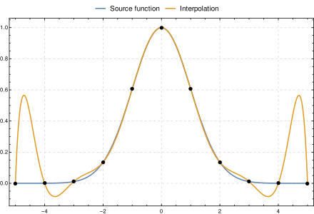
Lagrange and other interpolation at equally spaced points, as in the example above, yield a polynomial oscillating above and below the true function. This behaviour tends to grow with the number of points, leading to a divergence known as Runge's phenomenon; the problem may be eliminated by choosing interpolation points at Chebyshev nodes.[2]
The Lagrange basis polynomials can be used in numerical integration to derive the Newton–Cotes formulas.
Barycentric form
Using


we can rewrite the Lagrange basis polynomials as

or, by defining the barycentric weights[3]

we can simply write

which is commonly referred to as the first form of the barycentric interpolation formula.
The advantage of this representation is that the interpolation polynomial may now be evaluated as

which, if the weights have been pre-computed, requires only operations (evaluating and the weights ) as opposed to for evaluating the Lagrange basis polynomials individually.


The barycentric interpolation formula can also easily be updated to incorporate a new node by dividing each of the , by and constructing the new as above.


We can further simplify the first form by first considering the barycentric interpolation of the constant function :


Dividing by does not modify the interpolation, yet yields


which is referred to as the second form or true form of the barycentric interpolation formula. This second form has the advantage that need not be evaluated for each evaluation of .
Remainder in Lagrange interpolation formula
When interpolating a given function f by a polynomial of degree n at the nodes x0,...,xn we get the remainder which can be expressed as [4]

![R(x)=f[x_{0},\ldots ,x_{n},x]\ell (x)=\ell (x){\frac {f^{n+1}(\xi )}{(n+1)!}},\quad \quad x_{0}<\xi <x_{n},](../I/m/db5c9bccf5ba27de59d843f69da0b6e3fe560771.svg)
where and is the notation for divided differences. Alternatively, the remainder can be expressed as a contour integral in complex domain as
![f[x_{0},\ldots ,x_{n},x]](../I/m/19168012592a247cadfadee2ec1a0329c5288f1f.svg)

The remainder can be bound as

First derivative
The first derivative of the lagrange polynomial is given by

where .

Finite fields
The Lagrange polynomial can also be computed in finite fields. This has applications in cryptography, such as in Shamir's Secret Sharing scheme.
See also
- Neville's algorithm
- Newton form of the interpolation polynomial
- Bernstein form of the interpolation polynomial
- Carlson's theorem
- Lebesgue constant (interpolation)
- The Chebfun system
- Table of Newtonian series
- Frobenius covariant
- Sylvester's formula
References
- ↑ Meijering, Erik (2002), "A chronology of interpolation: from ancient astronomy to modern signal and image processing", Proceedings of the IEEE, 90 (3): 319–342, doi:10.1109/5.993400.
- ↑ Quarteroni, Alfio; Saleri, Fausto (2003), Scientific Computing with MATLAB, Texts in computational science and engineering, 2, Springer, p. 66, ISBN 9783540443636.
- ↑ Jean-Paul Berrut & Lloyd N. Trefethen (2004). "Barycentric Lagrange Interpolation". SIAM Review. 46 (3): 501–517. doi:10.1137/S0036144502417715.
- ↑ Abramowitz and Stegun, "Handbook of Mathematical Functions," p.878
External links
- Hazewinkel, Michiel, ed. (2001), "Lagrange interpolation formula", Encyclopedia of Mathematics, Springer, ISBN 978-1-55608-010-4
- ALGLIB has an implementations in C++ / C# / VBA / Pascal.
- GSL has a polynomial interpolation code in C
- SO has a MATLAB example that demonstrates the algorithm and recreates the first image in this article
- Lagrange Method of Interpolation — Notes, PPT, Mathcad, Mathematica, MATLAB, Maple at Holistic Numerical Methods Institute
- Lagrange interpolation polynomial on www.math-linux.com
- Weisstein, Eric W. "Lagrange Interpolating Polynomial". MathWorld.
- Estimate of the error in Lagrange Polynomial Approximation at ProofWiki
- Module for Lagrange Polynomials by John H. Mathews
- Dynamic Lagrange interpolation with JSXGraph
- Numerical computing with functions: The Chebfun Project
- Excel Worksheet Function for Bicubic Lagrange Interpolation
- Lagrange polynomials in Python