Marginal distribution

In probability theory and statistics, the marginal distribution of a subset of a collection of random variables is the probability distribution of the variables contained in the subset. It gives the probabilities of various values of the variables in the subset without reference to the values of the other variables. This contrasts with a conditional distribution, which gives the probabilities contingent upon the values of the other variables.

The term marginal variable is used to refer to those variables in the subset of variables being retained. These terms are dubbed "marginal" because they used to be found by summing values in a table along rows or columns, and writing the sum in the margins of the table.^[1] The distribution of the marginal variables (the marginal distribution) is obtained by marginalizing over the distribution of the variables being discarded, and the discarded variables are said to have been marginalized out.

The context here is that the theoretical studies being undertaken, or the data analysis being done, involves a wider set of random variables but that attention is being limited to a reduced number of those variables. In many applications an analysis may start with a given collection of random variables, then first extend the set by defining new ones (such as the sum of the original random variables) and finally reduce the number by placing interest in the marginal distribution of a subset (such as the sum). Several different analyses may be done, each treating a different subset of variables as the marginal variables.

Two-variable case

X Y	x1	x2	x3	x4	py(Y)↓
y1	^4⁄32	^2⁄32	^1⁄32	^1⁄32	^8⁄32
y2	^2⁄32	^4⁄32	^1⁄32	^1⁄32	^8⁄32
y3	^2⁄32	^2⁄32	^2⁄32	^2⁄32	^8⁄32
y4	^8⁄32	0	0	0	^8⁄32
px(X) →	^16⁄32	^8⁄32	^4⁄32	^4⁄32	^32⁄32
Joint and marginal distributions of a pair of discrete, random variables X,Y having nonzero mutual information I(X; Y). The values of the joint distribution are in the 4×4 square, and the values of the marginal distributions are along the right and bottom margins.

Given two random variables X and Y whose joint distribution is known, the marginal distribution of X is simply the probability distribution of X averaging over information about Y. It is the probability distribution of X when the value of Y is not known. This is typically calculated by summing or integrating the joint probability distribution over Y.

For discrete random variables, the marginal probability mass function can be written as Pr(X = x). This is

${\displaystyle \Pr(X=x)=\sum _{y}\Pr(X=x,Y=y)=\sum _{y}\Pr(X=x\mid Y=y)\Pr(Y=y),}$

where Pr(X = x,Y = y) is the joint distribution of X and Y, while Pr(X = x|Y = y) is the conditional distribution of X given Y. In this case, the variable Y has been marginalized out.

Bivariate marginal and joint probabilities for discrete random variables are often displayed as two-way tables.

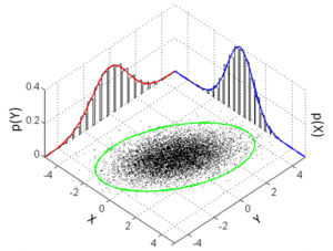
Similarly for continuous random variables, the marginal probability density function can be written as p_X(x). This is

${\displaystyle p_{X}(x)=\int _{y}p_{X,Y}(x,y)\,\mathrm {d} y=\int _{y}p_{X\mid Y}(x\mid y)\,p_{Y}(y)\,\mathrm {d} y,}$

where p_X,Y(x,y) gives the joint distribution of X and Y, while p_X|Y(x|y) gives the conditional distribution for X given Y. Again, the variable Y has been marginalized out.

Note that a marginal probability can always be written as an expected value:

${\displaystyle p_{X}(x)=\int _{y}p_{X\mid Y}(x\mid y)\,p_{Y}(y)\,\mathrm {d} y=\mathbb {E} _{Y}[p_{X\mid Y}(x\mid y)]}$

Intuitively, the marginal probability of X is computed by examining the conditional probability of X given a particular value of Y, and then averaging this conditional probability over the distribution of all values of Y.

This follows from the definition of expected value (after applying the Law of the unconscious statistician):

${\displaystyle \mathbb {E} _{Y}[f(Y)]=\int _{y}f(y)p_{Y}(y)\,\mathrm {d} y.}$

Therefore marginalization provides the rule for the transformation of the probability distribution of a random variable Y and another random variable X = g(Y):

${\displaystyle p_{X}(x)=\int _{y}p_{X\mid Y}(x\mid y)\,p_{Y}(y)\,\mathrm {d} y=\int _{y}\delta (x-g(y))\,p_{Y}(y)\,\mathrm {d} y,}$

Real-world example

Suppose that the probability that a pedestrian will be hit by a car while crossing the road at a pedestrian crossing without paying attention to the traffic light is to be computed. Let H be a discrete random variable taking one value from {Hit, Not Hit}. Let L be a discrete random variable taking one value from {Red, Yellow, Green}.

Realistically, H will be dependent on L. That is, P(H = Hit) and P(H = Not Hit) will take different values depending on whether L is red, yellow or green. A person is, for example, far more likely to be hit by a car when trying to cross while the lights for cross traffic are green than if they are red. In other words, for any given possible pair of values for H and L, one must consider the joint probability distribution of H and L to find the probability of that pair of events occurring together if the pedestrian ignores the state of the light.

However, in trying to calculate the marginal probability P(H=hit), what we are asking for is the probability that H=Hit in the situation in which we don't actually know the particular value of L and in which the pedestrian ignores the state of the light. In general a pedestrian can be hit if the lights are red OR if the lights are yellow OR if the lights are green. So in this case the answer for the marginal probability can be found by summing P(H,L) for all possible values of L, with each value of L weighted by its probability of occurring.

Here is a table showing the conditional probabilities of being hit, depending on the state of the lights. (Note that the columns in this table must add up to 1 because the probability of being hit or not hit is 1 regardless of the state of the light.)

Conditional distribution: ${\displaystyle P(H|L)}$

L H	Red	Yellow	Green
Not Hit	0.99	0.9	0.2
Hit	0.01	0.1	0.8

To find the joint probability distribution, we need more data. Let's say that P(L=red) = 0.2, P(L=yellow) = 0.1, and P(L=green) = 0.7. Multiplying each column in the conditional distribution by the probability of that column occurring, we find the joint probability distribution of H and L, given in the central 2×3 block of entries. (Note that the cells in this 2×3 block add up to 1).

Joint distribution: ${\displaystyle P(H,L)}$

L H	Red	Yellow	Green	Marginal probability P(H)
Not Hit	0.198	0.09	0.14	0.428
Hit	0.002	0.01	0.56	0.572
Total	0.2	0.1	0.7	1

The marginal probability P(H=Hit) is the sum along the H=Hit row of this joint distribution table, as this is the probability of being hit when the lights are red OR yellow OR green. Similarly, the marginal probability that P(H=Not Hit) is the sum of the H=Not Hit row. In this example the probability of a pedestrian being hit if they don't pay attention to the condition of the traffic light is 0.572.

Multivariate distributions

Many samples from a bivariate normal distribution. The marginal distributions are shown in red and blue. The marginal distribution of X is also approximated by creating a histogram of the X coordinates without consideration of the Y coordinates.

For multivariate distributions, formulae similar to those above apply with the symbols X and/or Y being interpreted as vectors. In particular, each summation or integration would be over all variables except those contained in X.

See also

• Joint probability distribution
• Wasserstein metric

References

1. Trumpler and Weaver (1962), pp. 32–33.

Bibliography

• Everitt, B. S. (2002). The Cambridge Dictionary of Statistics. Cambridge University Press. ISBN 0-521-81099-X.
• Trumpler, Robert J. and Harold F. Weaver (1962). Statistical Astronomy. Dover Publications.