Mathieu wavelet

The Mathieu equation is a linear second-order differential equation with periodic coefficients. The French mathematician, E. Léonard Mathieu, first introduced this family of differential equations, nowadays termed Mathieu equations, in his “Memoir on vibrations of an elliptic membrane” in 1868. "Mathieu functions are applicable to a wide variety of physical phenomena, e.g., diffraction, amplitude distortion, inverted pendulum, stability of a floating body, radio frequency quadrupole, and vibration in a medium with modulated density"^[1]

Elliptic-cylinder wavelets

This is a wide family of wavelet system that provides a multiresolution analysis. The magnitude of the detail and smoothing filters corresponds to first-kind Mathieu functions with odd characteristic exponent. The number of notches of these filters can be easily designed by choosing the characteristic exponent. Elliptic-cylinder wavelets derived by this method ^[2] possess potential application in the fields of optics and electromagnetism due to its symmetry.

Mathieu differential equations

Mathieu's equation is related to the wave equation for the elliptic cylinder. In 1868, the French mathematician Émile Léonard Mathieu introduced a family of differential equations nowadays termed Mathieu equations.^[3]

Given $a \in \mathbb{R}, q \in \mathbb{C}$, the Mathieu equation is given by

$\frac {d^2 y} {dw^2} +(a-2q \cos 2w )y=0.$

The Mathieu equation is a linear second-order differential equation with periodic coefficients. For q = 0, it reduces to the well-known harmonic oscillator, a being the square of the frequency.^[4]

The solution of the Mathieu equation is the elliptic-cylinder harmonic, known as Mathieu functions. They have long been applied on a broad scope of wave-guide problems involving elliptical geometry, including:

1. analysis for weak guiding for step index elliptical core optical fibres
2. power transport of elliptical wave guides
3. evaluating radiated waves of elliptical horn antennas
4. elliptical annular microstrip antennas with arbitrary eccentricity $\nu$)
5. scattering by a coated strip.

Mathieu functions: cosine-elliptic and sine-elliptic functions

In general, the solutions of Mathieu equation are not periodic. However, for a given q, periodic solutions exist for infinitely many special values (eigenvalues) of a. For several physically relevant solutions y must be periodic of period $\pi$ or $2\pi$. It is convenient to distinguish even and odd periodic solutions, which are termed Mathieu functions of first kind.

One of four simpler types can be considered: Periodic solution ($\pi$ or $2\pi$) symmetry (even or odd).

For $q \ne 0$, the only periodic solutions y corresponding to any characteristic value $a=a_r(q)$ or $a=b_r(q)$ have the following notations:

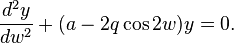
ce and se are abbreviations for cosine-elliptic and sine-elliptic, respectively.

• Even periodic solution:

$ce_r(\omega,q)= \sum_m A_{r,m} \cos {m \omega}\text{ for }a=a_r(q)$

• Odd periodic solution:

$se_r(\omega,q)= \sum_m A_{r,m} \sin {m \omega}\text{ for }a=b_r(q)$

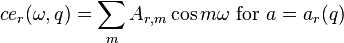
where the sums are taken over even (respectively odd) values of m if the period of y is $\pi$ (respectively $2\pi$).

Given r, we denote henceforth $A_{r,m}$ by $A_m$, for short.

Interesting relationships are found when $q \to 0$, $r \ne 0$:

$\lim_{q \to 0} ce_r(\omega,q)= \cos {r \omega}$

$\lim_{q \to 0} se_r(\omega,q)= \sin {r \omega}$

Figure 1 shows two illustrative waveform of elliptic cosines, whose shape strongly depends on the parameters $\nu$ and q.

Figure 1. Some plots of $2\pi$-periodic 1st kind even Mathieu functions. Elliptic cosines shape for the following set of parameters: a) $\nu=1$=and q = 5 ; b) $\nu=5$=and q = 5.

Multiresolution analysis filters and Mathieu's equation

Wavelets are denoted by $\psi(t)$ and scaling functions by $\phi(t)$, with corresponding spectra $\Psi(\omega)$ and $\Phi(\omega)$, respectively.

The equation 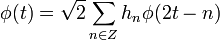$\phi(t)= \sqrt {2} \sum_{n \in Z} h_n \phi(2t-n)$, which is known as the dilation or refinement equation, is the chief relation determining a Multiresolution Analysis (MRA).

$H(\omega)= \frac {1} {\sqrt 2} \sum_{k \in Z} h_k e^{j \omega k}$ is the transfer function of the smoothing filter.

$G(\omega)= \frac {1} {\sqrt 2} \sum_{k \in Z} g_k e^{j \omega k}$ is the transfer function of the detail filter.

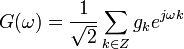
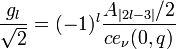
The transfer function of the "detail filter" of a Mathieu wavelet is

$G_{\nu}(\omega)=e^{j(\nu-2)[ \frac {\omega - \pi} {2}]}. \frac {ce_{\nu} ( \frac {\omega-\pi} {2},q)} {{ce_{\nu}(0,q)}}.$

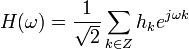
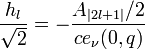
The transfer function of the "smoothing filter" of a Mathieu wavelet is

$H_{\nu}(\omega)=-e^{j\nu [ \frac {\omega} {2}]}. \frac {ce_{\nu}( \frac {\omega} {2},q)} {{ce_{\nu}(0,q)}}.$

The characteristic exponent $\nu$ should be chosen so as to guarantee suitable initial conditions, i.e. $G_{\nu}(0)=0$ and $G_{\nu}(\pi)=1$, which are compatible with wavelet filter requirements. Therefore, $\nu$ must be odd.

The magnitude of the transfer function corresponds exactly to the modulus of an elliptic-sine:

Examples of filter transfer function for a Mathieu MRA are shown in the figure 2. The value of a is adjusted to an eigenvalue in each case, leading to a periodic solution. Such solutions present a number of $\nu$ zeroes in the interval $0 \le |\omega | \le \pi$.

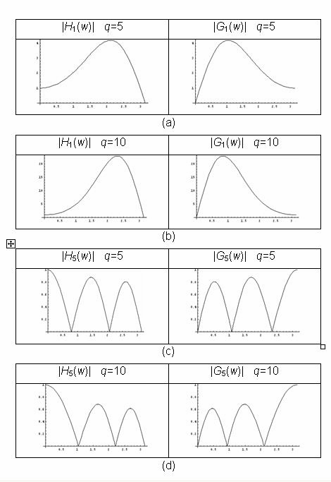
Figure 2 - Magnitude of the transfer function for Mathieu multiresolution analysis filters. (smoothing filter $H_{\nu}( \omega)$ and detail filter $G_{\nu}( \omega)$ for a few Mathieu parameters.) (a) $\nu=1$, q=5, a = 1.85818754...; (b) $\nu=1$, q = 10, a = −2.3991424...; (c) $\nu=5$, q = 10, a = 25.5499717...; (d) $\nu=5$, q = 10, a = 27.70376873...

The G and H filter coefficients of Mathieu MRA can be expressed in terms of the values $\{ A_{2 l +1} \}_{l \in Z}$ of the Mathieu function as:

$\frac {h_l} {\sqrt{2}}=- \frac {A_{|2l+1|}/2} {ce_{\nu}(0,q)}$

$\frac {g_l} {\sqrt{2}}=(-1)^l \frac {A_{|2l-3|}/2} {ce_{\nu}(0,q)}$

There exist recurrence relations among the coefficients:

$(a-1-q)A_1-qA_3 =0$

$(a-m^2)A_m-q(A_{m-2}+A_{m+2} =0$

for $m \ge 3$, m odd.

It is straightforward to show that $h_{-l}=h_{|l|-1}$, $\forall l>0$.

Normalising conditions are $\sum_{k=- \infty}^{k=+ \infty} {h_k =-1}$ and $\sum_{k=- \infty}^{k=+ \infty} {(-1)^k h_k =0}$.

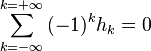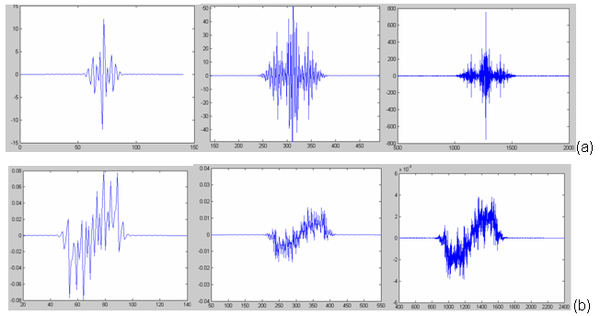
Waveform of Mathieu wavelets

Mathieu wavelets can be derived from the lowpass reconstruction filter by the cascade algorithm. Infinite Impulse Response filters (IIR filter) should be use since Mathieu wavelet has no compact support. Figure 3 shows emerging pattern that progressively looks like the wavelet's shape. Depending on the parameters a and q some waveforms (e.g. fig. 3b) can present a somewhat unusual shape.

Figure 3: FIR-based approximation of Mathieu wavelets. Filter coefficients holding h < 10⁻¹⁰ were thrown away (20 retained coefficients per filter in both cases.) (a) Mathieu Wavelet with ν = 5 and q = 5 and (b) Mathieu wavelet with ν = 1 and q = 5.

References

1. L. Ruby, “Applications of the Mathieu Equation,” Am. J. of Physics, vol. 64, pp. 39–44, Jan. 1996
2. M.M.S. Lira, H.M. de Oiveira, R.J.S. Cintra. Elliptic-Cylindrical Wavelets: The Mathieu Wavelets,IEEE Signal Processing Letters, vol.11, n.1, January, pp. 52–55, 2004.
3. É. Mathieu, Mémoire sur le mouvement vibratoire d'une membrane de forme elliptique, J. Math. Pures Appl., vol.13, 1868, pp. 137–203.
4. N.W. McLachlan, Theory and Application of Mathieu Functions, New York: Dover, 1964.