Multidimensional empirical mode decomposition
In signal processing, the multidimensional empirical mode decomposition (multidimensional EMD) is the extension of the 1-D EMD algorithm into multiple-dimensional signal. It is very advantageous to decompose a complex signal into simple signals without leaving the time domain. The Hilbert–Huang empirical mode decomposition (EMD) process decomposes signal into intrinsic mode functions combined with the Hilbert spectral analysis known as Hilbert–Huang transform (HHT). The multidimensional EMD extends the 1-D EMD algorithm into multiple-dimensional signals. This decomposition can be applied to image processing, audio signal processing and various other multidimensional signals.
Motivation
Multidimensional Empirical Mode Decomposition is a popular method because of its applications in many fields, such as texture analysis, financial applications, image processing, ocean engineering, seismic research and so on. Recently, several methods of Empirical Mode Decomposition have been used to collect the data and analyze characterization of multidimensional signals. In this article, we will introduce the basic of Multidimensional Empirical Mode Decomposition, and then look into the enhancing approach for traditional Multidimensional Empirical Mode Decomposition.
Introduction of empirical mode decomposition (EMD)
The Hilbert transform when applied for instantaneous frequency computation, the derived instantaneous frequency of the signal could lose its physical meaning when the signal is not an AM/FM separable oscillatory function. Due to those stable and capable properties of Empirical Mode Decomposition, the Empirical Mode Decomposition method can extract global structure and deal with fractal-like signal perfectly.
The EMD method was developed to overcome this drawback so that the data can be examined in a physically meaningful adaptive time–frequency–amplitude space for nonlinear and non-stationary signals.
The EMD method decomposes input signal into a few Intrinsic Mode functions (IMF). The multi-components signal decompose into intrinsic mode and a residue after IMFs formed. The given equation will be as follows:

where is the function of multi-components signal. is the Intrinsic Mode Function, and represents residue into intrinsic modes.


Ensemble empirical mode decomposition
The EEMD consists of the following steps:
- Adding a white noise series to the original data.
- Decomposing the data with added white noise into oscillatory components.
- Repeating step 1 and step 2 again and again, but with different white noise series added each time.
- Obtaining the (ensemble) means of the corresponding intrinsic mode functions of the decomposition as the final result.
In these steps, EEMD uses two properties of white noise:
- The added white noise leads to relatively even distribution of extrema distribution on all timescales.
- The dyadic filter bank property provides a control on the periods of oscillations contained in an oscillatory component, significantly reducing the chance of scale mixing in a component. Through ensemble average, the added noise is averaged out.[1]
Multi-dimension EEMD
Technique 1
[2] To design a MDEEMD algorithm the key step is to translate the algorithm of the 1D EMD into a Bi-dimensional Empirical Mode Decomposition(BEMD) and further extend the algorithm to three or more dimensions which is like the BEMD by extending the procedure on successive dimensions. Mathematically let us represent a 2D signal in the form of ixj matrix form with a finite number of elements.

First EMD is performed in one direction of X(i,j), Row wise for instance, to decompose the data of each row into m components, then to collect the components of the same level of m from the result of each row decomposition to make a 2D decomposed signal at that level of m. Therefore, m set of 2D spatial data are obtained
![{\displaystyle {\begin{aligned}RX(1,i,j)&={\begin{bmatrix}x(1,1,1)&x(1,1,2)&\cdots &x(1,1,j)\\x(1,2,1)&x(1,2,2)&\cdots &x(1,1,j)\\\vdots &\vdots &&\vdots \\x(1,i,1)&x(1,i,2)&\cdots &x(1,i,j)\end{bmatrix}}\\[6pt]RX(2,i,j)&={\begin{bmatrix}x(2,1,1)&x(2,1,2)&\cdots &x(2,1,j)\\x(2,2,1)&x(2,2,2)&\cdots &x(2,1,j)\\\vdots &\vdots &&\vdots \\x(2,i,1)&x(2,i,2)&\cdots &x(2,i,j)\end{bmatrix}}\\\vdots \qquad &\,\,\,\vdots \qquad \vdots \\[6pt]RX(m,i,j)&={\begin{bmatrix}x(m,1,1)&x(m,1,2)&\cdots &x(m,1,j)\\x(m,2,1)&x(m,2,2)&\cdots &x(m,1,j)\\\vdots &\vdots &&\vdots \\x(m,i,1)&x(m,i,2)&\cdots &x(m,i,j)\end{bmatrix}}\end{aligned}}}](../I/m/54a89e9bc9d72662fe1064efca887d4ae428f3b1.svg)
where RX (1, i, j), RX (2, i, j), and RX (m, i, j) are the m sets of signal as stated (also here we use R to indicate row decomposing). The relation between these m 2D decomposed signals and the original signal is given as [2]

The first row of the matrix RX (m, i, j) is the mth EMD component decomposed from the first row of the matrix X (i, j). The second row of the matrix RX (m, i, j) is the mth EMD component decomposed from the second row of the matrix X (i, j), and so on.
Suppose that the previous decomposition is along the horizontal direction, the next step is to decompose each one of the previously row decomposed components RX(m, i, j), in the vertical direction into n components. This step will generate n components from each RX component.
For example, the component
- RX(1,i,j) will be decomposed into CRX(1,1,i,j), CRX(1,2,i,j),…,CRX(1,n,i,j)
- RX(2,i,j) will be decomposed into CRX(2,1,i,j), CRX(2,2,i,j),…, CRX(2,n,i,j)
- RX(m,i,j) will be decomposed into CRX(m,1,i,j), CRX(m,2,i,j),…, CRX(m,n,i,j)
where C means column decomposing.Finally, the 2D decomposition will result into m× n matrices which are the 2D EEMD components of the original data X(i,j). The matrix expression for the result of the 2D decomposition is

where each element in the matrix CRX is an i × j sub-matrix representing a 2D EEMD decomposed component. We use the arguments (or suffixes) m and n to represent the component number of row decomposition and column decomposition, respectively rather than the subscripts indicating the row and the column of a matrix. Notice that the m and n indicate the number of components resulting from row(horizontal) decomposition and then column (vertical) decomposition, respectively.
By combining the components of the same scale or the comparable scales with minimal difference will yield a 2D feature with best physical significance. The components of the first row and the first column are approximately the same or comparable scale although their scales are increasing gradually along the row or column. Therefore, combining the components of the first row and the first column will obtain the first complete 2D component (C2D1). The subsequent process is to perform the same combination technique to the rest of the components.

Following the convention of 1D EMD, the last component of the complete 2D components is called residue. The decomposition strategy can be extended without difficulty to higher or any dimensional data. For a 3D data cube of i × j × k elements, the multidimensional EMD decomposition will yield detailed 3D components of m × n × q where m, n and q are the number of the IMFs decomposed from each dimension having i, j, and k elements, respectively.
The MDEEMD method has several advantages. For instance, the sifting procedure of the MDEEMD is a combination of one dimensional sifting. It employs 1D curve fitting in the sifting process of each dimension, and has no difficulty as encountered in the 2D EMD algorithms using surface fitting which has the problem of determining the saddle point as a local maximum or minimum.Sifting is the process which separates the IMF and repeats the process until the residue is obtained. The first step of performing sifting is to determine the upper and lower envelopes encompassing all the data by using the spline method. Sifting scheme for MDEMD is like the 1D sifting where the local mean of the standard EMD is replaced by the mean of multivariate envelope curves.
Technique 2
A Fast and efficient data analysis is very important for large sequences hence the MDEEMD focuses on two important things
- Data compression which involves decomposing data into simpler forms.[3]
- EEMD on the compressed data, this is the most challenging since on decomposing the compressed data there is a high probability to lose key information. Hence the EEMD must be both highly efficient and fast to process large amounts of data. A data compression method that uses principal component analysis (PCA) or also known as empirical orthogonal function (EOF) analysis or principal oscillation pattern analysis is used to compress data.[3]
Assume, we have a spatio-temporal data T (s, t), where s is spatial locations (not necessary one dimensional originally but needed to be rearranged into a single spatial dimension) from 1 to N and t temporal locations from 1 to M.
Using PCA/EOF, one can express T (s, t) into [3]

where, Yi(t) is the ith Principal Component(PC) and Vi(s) the ith Empirical Orthogonal Function(EOF). PCs and EOFs are often obtained by solving the eigen-value/eigen-vector problem of either temporal co-variance matrix or spatial co-variance matrix based on which dimension is smaller. The variance explained by one pair of PCA/EOF is its corresponding eigenvalue divided by the sum of all eigenvalues of the co-variance matrix.
If the data subjected to PCA/EOF is all white noise, all eigenvalues are theoretically equal and there is no preferred vector direction (the principal component) in PCA/EOF space. To retain most of the information of the data, one needs to retain almost all the PC's and EOF's, making the size of PCA/EOF expression even larger than that of the original. If the original data contain only one spatial structure and oscillate with time, then the original data can be expressed as the product of one PC and one EOF, implying that the original data of large size can be expressed by small size data without losing information, i.e. highly compressible.
The variability of a smaller region tends to be more spatio-temporally coherent than a bigger region containing that smaller region, and, therefore, it is expected that fewer PC/EOF components are required to account for a threshold level of variance hence onne way to improve the efficiency of the representation of data in terms of PC/EOF component is to divide the global spatial domain into a set of sub-regions. If we divide the original global spatial domain into n sub-regions containing N1, N2, . . . ,Nn spatial grids, respectively, with all Ni, where i=1, . . . , n, greater than M, we anticipate that the numbers of the retained PC/EOF pairs for all sub-regions K1, K2, . . . ,Kn are all smaller than K. Therefore, the compression rate of the spatial domain is as follows

Note that an optimized division and an optimized selection of PC/EOF pairs for each region would lead to a higher rate of compression.
Technique 3 (Division of a spatial-temporal signal into grids)
For a temporal signal of length M, the complexity of cubic spline sifting through its local extrema is about the order of M which is similar for the EEMD, as it only repeats the spline fitting operation with a number that is not dependent on M. However, as the sifting number (often selected as 10) and the ensemble number (often a few hundred) multiply to the spline sifting operations, hence the EEMD is time consuming compared with many other time series analysis methods such as Fourier Transforms and Wavelet Transforms.The MDEEMD employs EEMD decomposition of the time series at each division grids of the initial temporal signal, the EEMD operation is repeated by the number of total grid points of the domain. The idea of the fast MDEEMD is very simple. As PCA/EOF-based compression expressed the original data in terms of pairs of PCs and EOFs, through decomposing PCs, instead of time series of each grid, and using the corresponding spatial structure depicted by the corresponding EOFs, the computational burden can be significantly reduced.
The fast MDEEMD which includes the following steps:[3]
- All pairs of EOF's, Vi, and their corresponding PCs, Yi, of Spatio-Temporal data over a compressed sub-domain are computed.
- The number of pairs of PC/EOF that are retained in the compressed data is determined by the calculation of the accumulated total variance of leading EOF/PC pairs.
- Each PC Yi is decomposed using EEMD, i.e.

where c(j,i) represents simple oscillatory modes of certain frequencies and r(n,i) is the residual of the data Yi. The result of the ith MEEMD component Cj is obtained as .[3] In this compressed computation, we have used the approximate dyadic filter bank properties of EMD/EEMD.

Advantages
A detailed knowledge of the Intrinsic mode functions of a noise corrupted signal can help in estimating the significance of that mode. It is usually assumed that the first IMF captures most of the noise and hence from this IMF we could estimate the Noise level and estimate the noise corrupted signal eliminating the effects of noise approximately. This method is known as Denoising and Detrending. Another advantage of using the MDEEMD is that the mode mixing is reduced significantly due to the function of the EEMD.
The Denoising and Detrending strategy can be used for image processing to enhance an image and similarly it could be applied to Audio Signals to remove corrupted data in speech. The MDEEMD could be used to break down images and audio signals into IMF and based on the knowledge of the IMF perform necessary operations. The decomposition of an image is very advantageous for Radar-based application the decomposition of an image could reveal land mines etc.[3]
Parallel implementation of MEEMD
In MEEMD, although ample parallelism potentially exists in the ensemble dimension and/or the non-operating dimensions, several challenges still face a high performance MEEMD implantation.[4]
- Dynamic data variations: In EEMD, white noises change the number of extrema causing some irregularity and load imbalance, and thus slowing down the parallel execution.
- Stride memory accesses of high-dimensional data: High dimensional data are stored in non-continuous memory locations. Accesses along high dimensions are thus strided and uncoalesced, wasting available memory bandwidth.
- Limited resources to harness parallelism: While the independent EMDs and/or EEMDs comprising an MEEMD provide high parallelism, the computational capacities of multi-core and many-core processors may not be sufficient to fully exploit the inherent parallelism of MEEMD. Moreover, increased parallelism may increase memory requirements beyond the memory capacities of these processors.In MEEMD, when a high degree of parallelism is given by the ensemble dimension and/or the non-operating dimensions, the benefits of using a thread-level parallel algorithm are threefold.[4]
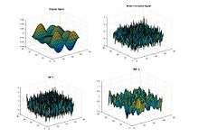
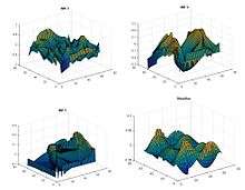 Bi-Dimensional EMD Intrinsic mode function along with the residue eliminating the noise level.
- It can exploit more parallelism than a block-level parallel algorithm.
- It does not incur any communication or synchronization between the threads until the results are merged since the execution of each EMD or EEMD is independent.
- Its implementation is like the sequential one, which makes it more straightforward.
OpenMp implementation
The EEMDs comprising MEEMD are assigned to independent threads for parallel execution, relying on the OpenMP runtime to resolve any load imbalance issues. Stride memory accesses of high-dimensional data are eliminated by transposing these data to lower dimensions, resulting in better utilization of cache lines. The partial results of each EEMD are made thread-private for correct functionality. The required memory depends on the number of OpenMP threads and is managed by OpenMP runtime.[4]
CUDA implementation
In the GPU CUDA implementation, each EMD, is mapped to a thread. The memory layout, especially of high-dimensional data, is rearranged to meet memory coalescing requirements and fit into the 128-byte cache lines. The data is first loaded along the lowest dimension and then consumed along a higher dimension. This step is performed when the Gaussian noise is added to form the ensemble data. In the new memory layout, the ensemble dimension is added to the lowest dimension to reduce possible branch divergence. The impact of the unavoidable branch divergence from data irregularity, caused by the noise, is minimized via a regularization technique using the on-chip memory. Moreover, the cache memory is utilized to amortize unavoidable uncoalesced memory accesses.[4]
Fast and adaptive multidimensional empirical mode decomposition
Concept
The Fast and Adaptive Bidimensional Empirical Mode Decomposition(FABEMD) is an improving version of traditional BEMD. The FABEMD can be used on many area, including medical image analysis, texture analysis and so on. Because of the difficulties facing in doing BEMD, the order statistics filter can help us solving the problems of efficiency and restriction of size in BEMD.
Based on the algorithm of BEMD, the implementation method of FABEMD is really similar to BEMD, but FABEMD approach just changes the interpolation step into a direct envelop estimation method and restrict the number of iteration for every BIMF to one. As a result, two order statistics, including MAX and MIN, will be used for approximate the upper and lower envelope. Otherwise, the size of the filter will depend on the maxima and minima maps obtained from input. The steps of FABEMD algorithm will be shown below.
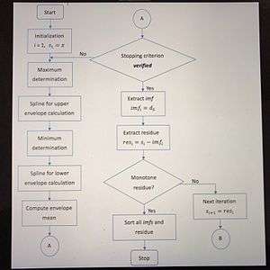
FABEMD algorithm[5]
- Step 1 – Determine and detect local maximum and minimum
As the traditional BEMD approach, we can find the jth ITS-BIMF of any source of input by neighboring window method. For FABEMD approach, we choose different way to implement.


From the input data, we can get an 2D matrix represent

where is the element location in the matrix A, and we can define the window size to be . Thus, we can obtain the maximum and minimum value from the matrix as follows:


where


- Step 2 – Obtain the size of window for order-statistic filter
At first, we define and to be the maximum and minimum distance in the array which is calculated from each local maximum or minimum point to the nearest nonzero element. Also, and will be sorted in descending order in the array according to the convenient selection. Otherwise, we will only consider square window. Thus, the selected equation for the gross window width as follows:


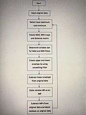


- Step 3 – Apply order statistics and smoothing filters to obtain the MAX and MIN filter output
To obtain the upper and lower envelopes, there should be defined two parameter and , and the equation will be as follows:


where is defined as the square region of window size, and is the window width of the smoothing filter which equals to . Therefore, the MAX and MIN filter will form a new 2-D matrix for envelope surface which will not change the original 2-D input data.[6]


- Step 4 – Set up an estimation from upper and lower envelopes
This step is to make sure that the envelope estimation in FABEMD is nearly closed to the result from BEMD by using interpolation. In order to do comparison, we need to form corresponding matrices for upper envelope, lower envelope and mean envelope by using thin-plate spline surface interpolation to the max and min maps.
Advantages
This method(FABEMD) provides a way to use less computation to obtain the result rapidly, and it allows us to ensure more accurate estimation of the BIMFs. Even more, the FABEMD is more adaptive to handle the large size input than tradition BEMD. Otherwise, the FABEMD is an efficient method that we do not need to consider the boundary effects and overshoot-undershoot problems.
Limitations
There is one particular problem that we will face in this method. Sometimes, there will be only one local maxima or minima element in the input data, so it will cause the distance array to be empty.
Partial differential equation-based multidimensional empirical mode decomposition
Concept
The Partial Differential Equation-Based Multidimensional Empirical Mode Decomposition(PDE-based MEMD) approach is a way to improve and overcome the difficulties of mean-envelope estimation of a signal from the traditional EMD. The PDE-based MEMD focus on modifying the original algorithm for MEMD. Thus, the result will provide an analytical formulation which can access to theoretical analysis and performance observation. In order to perform multidimensional EMD, we need to extend 1-D PDE-based sifting process to 2-D space. Then, the following steps will be shown below.
Here, we take 2-D PDE-based EMD for an example. The PDE-based BEMD consists steps as follows.
PDE-based BEMD algorithm[7]
- Step 1 – Extend super diffusion model from 1-D to 2-D
Considered a super diffusion matrix function

where represent the qth-order stopping function in direction i.

Then, the diffusion equation will be

where is the tension parameter, and we assumed that .


- Step 2 – Connect the relationship between diffusion model and PDEs on implicit surface
In order to make relationship to PDEs, the given equation will be

where is the 2qth-order differential operator on u intrinsic to surface S, and the initial condition for the equation will be for any y on surface S.


- Step 3 – Consider all the numerical resolutions
To obtain the theoretical and analysis result from the previous equation, we need to make an assumption.
Assumption:
Assumed that the numerical resolution schemes to be 4th-order PDE with no tension, and the equation for 4th-order PDE will be

First of all, we will explicit scheme by approximating the PDE-based sifting process.

where is a vector which consists the value of each pixel, is a matrix which is a difference approximation to the operator, and is a small time step.


Secondly, we can use AOS scheme to improve the property of stability, because the small time step will be unstable when it comes to large time step.
Finally, we can alternate direction implicit scheme. By using ADI-type schemes, it's suggested that to mix derivative term to overcome the problem that ADI-type schemes can only be used in second-order diffusion equation. The numerically solved equation will be followed

where is a matrix which is central difference approximation to the operator


Advantages
Based on the Navier-Strokes equations directly, this approach provides good way to obtain and develop with theoretical and numerical results. In particular, the PDE-based BEMD can well work on image decomposition fields. This approach can be applied on extracting transient signal and avoiding the indeterminacy characterization in some signals.
Boundary processing in bidimensional empirical decomposition by using texture synthesis
Concept
There are some problems in BEMD and boundary extending implementation in the iterative sifting process, including time consuming, shape and continuity of the edges, decomposition results comparison and so on. All these problems will cause decomposition useless. In order to fix these problems, the Boundary Processing in Bidimensional Empirical Decomposition by using Texture Synthesis (BPBEMD) method was created. The points of the new method algorithm will be shown as follows.
BPBEMD algorithm[8]
The few core steps for BPBEMD algorithm will be
- Step 1
Supposed the size of original input data and resultant data to be and , we can also define that original input data matrix will be in the middle of resultant data matrix.


- Step 2
Divided both original input data matrix and resultant data matrix in to block of size.

- Step 3
Find the block which is the most similar to their neighbor block in the Original input data matrix, and put it into the corresponding resultant data matrix.
- Step 4
Form a distance matrix which is weighted on the distance of different importance between each block from those boundaries.
- Step 5
Implemented iterative extension when it faces a huge boundary extension, we can seem that the block in original input data matrix is as the block in resultant data matrix.
Otherwise, there are two points we should take into consideration when we implement this method in image processing.[8]
- According to the different property between natural image and texture, we should notice that the local average intensity will easily change in every different images.
- In texture analysis, local contrast will be the same mostly if we analyze the same texture, but it may be different when we analyze a natural image.
Advantages
This method can process larger number of elements than traditional BEMD method. Also, it can shorten the time consuming for the process. Depended on using nonparametric sampling based texture synthesis, the BPBEMD could obtain better result after decomposing and extracting.
Limitations
Because most of image inputs are non-stationary which don’t exist boundary problems, the BPBEMD method is still lack of enough evidence that it is adaptive to all kinds of input data. Also, this method is narrowly restricted to be use on texture analysis and image processing.
Applications
In the first part, these MEEMD techniques can be used on the Geophysical data sets such as climate, magnetic, seismic data variability which takes advantage of the fast algorithm of MEEMD. The MEEMD is often used in the nonlinear geophysical data filtering due to its fast algorithms and its ability to handle large amount of data sets with the use of compression without losing and key information. The IMF can also be used as a signal enhancement of Ground Penetrating Radar for nonlinear data processing, it is very effective to detect geological boundaries from the analysis of field anomalies.
[9]
In the second part, the PDE-based MEMD and FAMEMD can be implemented on audio processing, image processing and texture analysis. Because of its several properties, including stability, less time consuming and so on, PDE-based MEMD method well works on adaptive decomposition, analyze texture and denoise data. Otherwise, the FAMEMD is a great method to reduce computation time and have more precise estimation in the process, so it will also be a certain method to implement audio processing, image processing and other more analysis. Finally, the BPBEMD method has well performance on image processing and texture analysis due to its property which is better to solve the extension boundary problems in recent techniques.
References
- ↑ N.E. Huang, Z. Shen, et al., "The Empirical Mode Decomposition and the Hilbert Spectrum for Nonlinear and Non- Stationary Time Series Analysis," Proceedings: Mathematical, Physical and Engineering Sciences, vol. 454, pp. 903-995, 1998.
- 1 2 3 4 5 6 Chih-Sung Chen, Yih Jeng, Department of Earth Sciences, National Taiwan Normal University, 88, Sec. 4, Ting-Chou Road, Taipei, 116, Taiwan, ROC, Two-dimensional nonlinear geophysical data filtering using the multidimensional EEMD method.
- 1 2 3 4 5 6 7 8 Wu Z, Feng J, Qiao F, Tan Z-M. 2016 Fast multidimensional ensemble empirical mode decomposition for the analysis of big spatio-temporal datasets. Phil. Trans. R. Soc. A 374: 20150197.
- 1 2 3 4 Li-Wen Chang, Men-Tzung Lo, Nasser Anssari, Ke-Hsin Hsu, Norden E. Huang, Wen-mei W. Hwu. Parallel implementation of Multidimensional Ensemble Mode Decomposition.
- 1 2 3 4 5 6 7 8 9 10 11 Sharif M. A. Bhuiyan, Reza R. Adhami, Jesmin F. Khan, "A Novel Approach of Fast and Adaptive Bidimensional Empirical Mode Decomposition", Acoustics, Speech and Signal Processing, 2008. ICASSP 2008. IEEE International Conference
- ↑ David Looney and Danilo P. Mandic, " Multiscale Image Fusion Using Complex Extensions of EMD", IEEE transactions on signal processing, Vol. 57, No. 4, Apirl 2009
- 1 2 3 4 5 6 7 Oumar Niang, Abdoulaye Thioune, Mouhamed Cheikh El Gueirea, Eric Deléchelle, and Jacques Lemoine, "Partial Differential Equation-Based Approach for Empirical Mode Decomposition: Application on Image Analysis", IEEE transactions on image processing, Vol. 21, No. 9, September 2012
- 1 2 Zhongxuan Liu and Silong Peng, "Boundary Processing of Bidimensional EMD Using Texture Synthesis", IEEE Signal Processing Letters, Vol. 12, No. 1, January 2005
- ↑ Bhuiyan, S.M.A., Attoh-Okine, N.O., Barner, K.E., Ayenu, A.Y., Adhami, R.R., 2009. Bidimensional empirical mode decomposition using various interpolation techniques. Adv. Adapt. Data Anal. 1, 309–338.