Simulation-based optimization

Simulation-based optimization integrates optimization techniques into simulation analysis. Because of the complexity of the simulation, the objective function may become difficult and expensive to evaluate.

Once a system is mathematically modeled, computer-based simulations provide the information about its behavior. Parametric simulation methods can be used to improve the performance of a system. In this method, the input of each variable is varied with other parameters remaining constant and the effect on the design objective is observed. This is a time-consuming method and improves the performance partially. To obtain the optimal solution with minimum computation and time, the problem is solved iteratively where in each iteration the solution moves closer to the optimum solution. Such methods are known as ‘numerical optimization’ or ‘simulation-based optimization’.^[1]

In simulation experiment, the goal is to evaluate the effect of different values of input variables on a system, which is called running simulation experiments. However the interest is sometimes in finding the optimal value for input variables in terms of the system outcomes. One way could be running simulation experiments for all possible input variables. However this approach is not always practical due to several possible situations and it just makes it intractable to run experiment for each scenario. For example, there might be so many possible values for input variables, or simulation model might be so complicated and expensive to run for suboptimal input variable values. In these cases, the goal is to find optimal values for input variables rather than trying all possible values. This process is called simulation optimization.^[2]

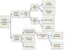
Specific simulation based optimization methods can be chosen according to figure 1 based on the decision variable types.^[3]

Fig.1 Classification of simulation based optimization according to variable types

Optimization exists in two main branches of operational research:

Optimization parametric (static) – the objective is to find the values of the parameters, which are “static” for all states, with the goal of maximize or minimize a function. In this case, there is the use of mathematical programming, such as linear programing. In this scenario, simulation helps when the parameters contain noise or the evaluation of the problem would demand excess of computer time, due to its complexity.^[4]

Optimization control (dynamic) – used largely in computer sciences and electrical engineering, what results in many papers and projects in these fields. The optimal control is per state and the results change in each of them. There is use of mathematical programming, as well as dynamic programming. In this scenario, simulation can generate random samples and solve complex and large-scale problems.^[4]

Simulation-based optimization methods

The main approaches in simulation optimization are discussed below. ^[5]

Statistical ranking and selection methods (R/S)

Ranking and selection methods are designed for problems where the alternatives are fixed and known, and simulation is used to estimate the system performance. In the simulation optimization setting, applicable methods include indifference zone approaches, optimal computing budget allocation, and knowledge gradient algorithms.

Response surface methodology (RSM)

In response surface methodology, the objective is to find the relationship between the input variables and the response variables. The process starts from trying to fit a linear regression model. If the P-value turns out to be low, then a higher degree polynomial regression, which is usually quadratic, will be implemented. The process of finding a good relationship between input and response variables will be done for each simulation test. In simulation optimization, response surface method can be used to find the best input variables that produce desired outcomes in terms of response variables.^[6]

Heuristic methods

Heuristic methods change accuracy by speed. Their goal is to find a good solution faster than the traditional methods, when they are too slow or fail in solving the problem. Usually they find local optimal instead of the optimal value; however, the values are considered close enough of the final solution. Examples of this kind of method is tabu search or Genetic algorithm.^[4]

Stochastic approximation

Stochastic approximation is used when the function cannot be computed directly, only estimated via noisy observations. In this scenarios, this method (or family of methods) looks for the extrema of these function. The objective function would be:^[7]

${\displaystyle {\underset {{\text{x}}\in \theta }{\min }}f{\bigl (}{\text{x}}{\bigr )}={\underset {{\text{x}}\in \theta }{\min }}\mathrm {E} [F{\bigl (}{\text{x,y}})]}$

$y$ is a random variable that represents the noise.

$x$ is the parameter that minimizes ${\displaystyle f{\bigl (}{\text{x}}{\bigr )}}$.

$\theta$ is the domain of the parameter $x$.

Derivative-free optimization methods

Derivative-free optimization is a subject of mathematical optimization. This method is applied to a certain optimization problem when its derivatives are unavailable or unreliable. Derivate-free method establishes model based on sample function values or directly draw a sample set of function values without exploiting detailed model. Since it needs no derivatives, it cannot be compared to derivative-based methods.[8]

For unconstrained optimization problems, it has a form:

${\displaystyle {\underset {{\text{x}}\in \mathbb {R} ^{n}}{\min }}f{\bigl (}{\text{x}}{\bigr )}}$

The limitation of derivative-free optimization:

1. It is usually cannot handle optimization problems with a few tens of variables, the results via this method are usually not so accurate.

2. When confronted with minimizing non-convex functions, it will show its limitation.

3. Derivative-free optimization methods is simple and easy, however, it is not so good in theory and in practice.

Dynamic programming and neuro-dynamic programming

Dynamic programming

Dynamic programming deals with situations where decisions are made in stage. The key to this kind of problems is to trade off the present and future costs.^[9]

One dynamic basic model has two features:

1) Has a discrete time dynamic system.

2) The cost function is additive over time.

For discrete feature, dynamic programming has the form:

${\displaystyle x_{k+1}=f_{k}(x_{k},u_{k},w_{k}),k=0,1,...,N-1}$

$k$ represents the index of discrete time.

$x_{k}$ is the state of the time k, it contains the past information and prepare it for the future optimization.

$u_{k}$ is the control variable.

$w_k$ is the random parameter.

For cost function, it has the form:

${\displaystyle g_{N}(X_{N})+\sum _{k=0}^{N-1}gk(x_{k},u_{k},W_{k})}$

${\displaystyle g_{N}(X_{N})}$ is the cost at the end of the process.

As the cost cannot be optimized meaningfully, it can be used the expect value:

${\displaystyle E\{g_{N}(X_{N})+\sum _{k=0}^{N-1}g_{k}(x_{k},u_{k},W_{k})\}}$

Neuro-dynamic programming

Neuro-dynamic programming is the same as dynamic programming except that the former has the concept of approximation architectures. It combines Artificial intelligence, simulation-base algorithms, and functional approach techniques. “Neuro” in this term origins from artificial intelligence community. It means learning how to make improved decisions for the future via built-in mechanism based on the current behavior. The most important part of neuro-dynamic programming is to build a trained neuro network for the optimal problem.^[10]

Limitations

Simulation based optimization has some limitations, such as the difficulty of creating a model that imitates the dynamic behavior of a system in a way that is considered good enough for its representation. Other problem is complexity in the determining uncontrollable parameters of both real-world system and simulation. Moreover, only a statistical estimation of real values can be obtained. It is not easy to determine the objective function, since it is a result of measurements, which can be harmful for the solutions.^[11][12]

References

1. Nguyen, Anh-Tuan, Sigrid Reiter, and Philippe Rigo. "A review on simulation-based optimization methods applied to building performance analysis."Applied Energy 113 (2014): 1043–1058.
2. Carson, Yolanda, and Anu Maria. "Simulation optimization: methods and applications." Proceedings of the 29th conference on Winter simulation. IEEE Computer Society, 1997.
3. Jalali, Hamed, and Inneke Van Nieuwenhuyse. "Simulation optimization in inventory replenishment: a classification." IIE Transactions 47.11 (2015): 1217-1235.
4. Abhijit Gosavi, Simulation‐Based Optimization: Parametric Optimization Techniques and Reinforcement Learning, Springer, 2nd Edition (2015)
5. Fu, Michael, editor (2015). Handbook of Simulation Optimization. Springer.
6. Rahimi Mazrae Shahi, M., Fallah Mehdipour, E. and Amiri, M. (2016), Optimization using simulation and response surface methodology with an application on subway train scheduling. Intl. Trans. in Op. Res., 23: 797–811. doi:10.1111/itor.12150
7. Powell, W. (2011). Approximate Dynamic Programming Solving the Curses of Dimensionality (2nd ed., Wiley Series in Probability and Statistics). Hoboken: Wiley.
8. Conn, A. R.; Scheinberg, K.; Vicente, L. N. (2009). Introduction to Derivative-Free Optimization. MPS-SIAM Book Series on Optimization. Philadelphia: SIAM. Retrieved 2014-01-18.
9. Cooper, Leon; Cooper, Mary W. Introduction to dynamic programming. New York: Pergamon Press, 1981
10. Van Roy, B., Bertsekas, D., Lee, Y., & Tsitsiklis, J. (1997). Neuro-dynamic programming approach to retailer inventory management. Proceedings of the IEEE Conference on Decision and Control, 4, 4052-4057.
11. Prasetio, Y. (2005). Simulation-based optimization for complex stochastic systems. University of Washington.
12. Deng, G., & Ferris, Michael. (2007). Simulation-based Optimization, ProQuest Dissertations and Theses