Stopping time

Example of a stopping time: a hitting time of Brownian motion. The process starts at 0 and is stopped as soon as it hits 1.

In probability theory, in particular in the study of stochastic processes, a stopping time (also Markov time) is a specific type of “random time”: a random variable whose value is interpreted as the time at which a given stochastic process exhibits a certain behavior of interest. A stopping time is often defined by a stopping rule, a mechanism for deciding whether to continue or stop a process on the basis of the present position and past events, and which will almost always lead to a decision to stop at some finite time.

Stopping times occur in decision theory, and the optional stopping theorem is an important result in this context. Stopping times are also frequently applied in mathematical proofs to “tame the continuum of time”, as Chung put it in his book (1982).

Definition

A stopping time with respect to a sequence of random variables X₁, X₂, ... is a random variable τ with values in {1,2,...} and the property that for each t∈{1,2,...}, the occurrence or non-occurrence of the event τ = t depends only on the values of X₁, X₂, ..., X_t. In some cases, the definition specifies that Pr(τ < ∞) = 1, or that τ be almost surely finite, although in other cases this requirement is omitted.

Another, more general definition is used for continuous-time stochastic processes and may be given in terms of a filtration: Let (I, ≤) be an ordered index set (often I = [0, ∞) or a compact subset thereof, thought of as the set of possible "times"), and let $(\Omega ,{\mathcal {F}},\{{\mathcal {F}}_{t}\}_{t\in I},\mathbb {P} )$ be a filtered probability space, i.e. a probability space equipped with a filtration of σ-algebras. Then a random variable $\tau$ : Ω → I is called a stopping time if $\{\omega \in \Omega :\tau (\omega )\leq t\}\in {\mathcal {F}}_{t}$ for all t in I.^[1] Often, to avoid confusion, we call it a ${\mathcal {F}}_{t}$ -stopping time and explicitly specify the filtration. Speaking intuitively, for $\tau$ to be a stopping time, it should be possible to decide whether or not $\{\tau \leq t\}$ has occurred on the basis of the knowledge of ${\mathcal {F}}_{t}$ , i.e., event $\{\tau \leq t\}$ is ${\mathcal {F}}_{t}$ -measurable.

Examples

To illustrate some examples of random times that are stopping rules and some that are not, consider a gambler playing roulette with a typical house edge, starting with $100 and betting $1 on red in each game:

Playing exactly five games corresponds to the stopping time τ = 5, and is a stopping rule.
Playing until he either runs out of money or has played 500 games is a stopping rule.
Playing until he is the maximum amount ahead he will ever be is not a stopping rule and does not provide a stopping time, as it requires information about the future as well as the present and past.
Playing until he doubles his money (borrowing if necessary if he goes into debt) is not a stopping rule, as there is a positive probability that he will never double his money.
Playing until he either doubles his money or runs out of money is a stopping rule, even though there is potentially no limit to the number of games he plays, since the probability that he stops in a finite time is 1.

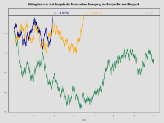
To illustrate the more general definition of stopping time, consider Brownian motion, which is a stochastic process $(B_{t})_{t\geq 0}$ , where each $B_{t}$ is a random variable defined on the probability space $(\Omega ,{\mathcal {F}},\mathbb {P} )$ . We define a filtration on this probability space by letting ${\mathcal {F}}_{t}$ be the σ-algebra generated by all the sets of the form $(B_{s})^{-1}(A)$ where $0\leq s\leq t$ and $A\subseteq \mathbb {R}$ is a Borel set. Intuitively, an event E is in ${\mathcal {F}}_{t}$ if and only if we can determine whether E is true or false just by observing the Brownian motion from time 0 to time t.

Every constant $\tau :=t_{0}$ is (trivially) a stopping time; it corresponds to the stopping rule "stop at time $t_{0}$ ".
Let $a\in \mathbb {R} .$ Then $\tau :=\inf\{t\geq 0\,|\,B_{t}>a\}$ is a stopping time for Brownian motion, corresponding to the stopping rule: "stop as soon as the Brownian motion exceeds the value a."
Another stopping time is given by $\tau :=\inf\{t\geq 1\,|\,B_{s}>0{\text{ for all }}s\in [t-1,t]\}$ . It corresponds to the stopping rule "stop as soon as the Brownian motion has been positive over a contiguous stretch of length 1 time unit."
In general, if τ₁ and τ₂ are stopping times on $\left(\Omega ,{\mathcal {F}},\left\{{\mathcal {F}}_{t}\right\}_{t\geq 0},\mathbb {P} \right)$ then their minimum $\tau _{1}\wedge \tau _{2}$ , their maximum $\tau _{1}\vee \tau _{2}$ , and their sum τ₁ + τ₂ are also stopping times. (This is not true for differences and products, because these may require "looking into the future" to determine when to stop.)

Hitting times like the second example above can be important examples of stopping times. While it is relatively straightforward to show that essentially all stopping times are hitting times,^[2] it can be much more difficult to show that a certain hitting time is a stopping time. The latter types of results are known as the Début theorem.

Localization

Stopping times are frequently used to generalize certain properties of stochastic processes to situations in which the required property is satisfied in only a local sense. First, if X is a process and τ is a stopping time, then X^τ is used to denote the process X stopped at time τ.

X_{t}^{\tau }=X_{\min(t,\tau )}

Then, X is said to locally satisfy some property P if there exists a sequence of stopping times τ_n, which increases to infinity and for which the processes

\mathbf {1} _{\{\tau _{n}>0\}}X^{\tau _{n}}

satisfy property P. Common examples, with time index set I = [0, ∞), are as follows:

Local Martingale Process. A process X is a local martingale if it is càdlàg and there exists a sequence of stopping times τ_n increasing to infinity, such that
$\mathbf {1} _{\{\tau _{n}>0\}}X^{\tau _{n}}$
is a martingale for each n.

Locally Integrable Process. A non-negative and increasing process X is locally integrable if there exists a sequence of stopping times τ_n increasing to infinity, such that
$\mathbb {E} \left[\mathbf {1} _{\{\tau _{n}>0\}}X^{\tau _{n}}\right]<\infty$
for each n.

Types of stopping times

Stopping times, with time index set I = [0,∞), are often divided into one of several types depending on whether it is possible to predict when they are about to occur.

A stopping time τ is predictable if it is equal to the limit of an increasing sequence of stopping times τ_n satisfying τ_n < τ whenever τ > 0. The sequence τ_n is said to announce τ, and predictable stopping times are sometimes known as announceable. Examples of predictable stopping times are hitting times of continuous and adapted processes. If τ is the first time at which a continuous and real valued process X is equal to some value a, then it is announced by the sequence τ_n, where τ_n is the first time at which X is within a distance of 1/n of a.

Accessible stopping times are those that can be covered by a sequence of predictable times. That is, stopping time τ is accessible if, P(τ = τ_n for some n) = 1, where τ_n are predictable times.

A stopping time τ is totally inaccessible if it can never be announced by an increasing sequence of stopping times. Equivalently, P(τ = σ < ∞) = 0 for every predictable time σ. Examples of totally inaccessible stopping times include the jump times of Poisson processes.

Every stopping time τ can be uniquely decomposed into an accessible and totally inaccessible time. That is, there exists a unique accessible stopping time σ and totally inaccessible time υ such that τ = σ whenever σ < ∞, τ = υ whenever υ < ∞, and τ = ∞ whenever σ = υ = ∞. Note that in the statement of this decomposition result, stopping times do not have to be almost surely finite, and can equal ∞.

References

↑ Duffie (2001): Asset Pricing Theory, Princeton University Press, page 324f.
↑ Fischer, Tom (2013). "On simple representations of stopping times and stopping time sigma-algebras". Statistics and Probability Letters. 83 (1): 345–349. doi:10.1016/j.spl.2012.09.024.