APL syntax and symbols
The APL programming language is distinctive in being symbolic rather than lexical: its primitives are denoted by symbols, not words. These symbols were originally devised as a mathematical notation. APL programmers often assign informal names when discussing functions and operators (for example, product for ×/) but the core functions and operators provided by the language are denoted by non-textual symbols.
Monadic and dyadic functions
Most symbols denote functions or operators. A monadic function takes as its argument the result of evaluating everything to its right. (Moderated in the usual way by parentheses.) A dyadic function has another argument, the first item of data on its left. Many symbols denote both monadic and dyadic functions, interpreted according to use. For example, ⌊3.2 gives 3, the largest integer not above the argument, and 3⌊2 gives 2, the lower of the two arguments.
Functions and operators
APL uses the term operator in Heaviside’s sense as a moderator of a function as opposed to some other programming language's use of the same term as something that operates on data, ref. relational operator and operators generally. Other programming languages also sometimes use this term interchangeably with function, however both terms are used in APL more precisely.[1][2][3][4][5] Early definitions of APL symbols were very specific about how symbols were categorized, ref. IBM's 5100 APL Reference Manual, first edition, circa 1975.[6] For example, the operator reduce is denoted by a forward slash and reduces an array along one axis by interposing its function operand. An example of reduce:
×/2 3 4 24 |
<< Equivalent results in APL >> << Reduce operator / used at left |
2×3×4 24 |
In the above case, the reduce or slash operator moderates the multiply function. The expression ×/2 3 4 evaluates to a scalar (1 element only) result through reducing an array by multiplication. The above case is simplified, imagine multiplying (adding, subtracting or dividing) more than just a few numbers together. (From a vector, ×/ returns the product of all its elements.)
1 0 1\45 67 45 0 67 |
<< Opposite results in APL >> << Expand dyadic function \ used at left Reduce dyadic function / used at right >> |
1 0 1/45 0 67 45 67 |
The above dyadic functions examples [left and right examples] (using the same / symbol, right example) demonstrate how boolean values (0s and 1s) can be used as left arguments for the \ expand and / replicate functions to produce exactly opposite results. On the left side, the 2-element vector {45 67} is expanded where boolean 0s occur to result in a 3-element vector {45 0 67} - note how APL inserted a 0 into the vector. Conversely, the exact opposite occurs on the right side - where a 3-element vector becomes just 2-elements; boolean 0s delete items using the dyadic / slash function. APL symbols also operate on lists (vector) of items using data types other than just numeric, for example a 2-element vector of character strings {"Apples" "Oranges"} could be substituted for numeric vector {45 67} above.
Syntax rules
In APL there is no precedence hierarchy for functions or operators. APL's syntax rule is therefore different from what is taught in mathematics where, for example multiplication is performed before addition, under order of operations.
The scope of a function determines its arguments. Functions have long right scope: that is, they take as right arguments everything to their right. A dyadic function has short left scope: it takes as its left arguments the first piece of data to its left. For example(leftmost column below is actual program code from an APL user session, indented = actual user input, not-indented = result returned by APL interpreter):
      1 ÷ 2 ⌊ 3 × 4 - 5
¯0.3333333333
      1 ÷ 2 ⌊ 3 × ¯1
¯0.3333333333
      1 ÷ 2 ⌊ ¯3
¯0.3333333333
      1 ÷ ¯3
¯0.3333333333
|
<< First note there are no parentheses and Step 2) 3 times -1 = -3. |
An operator may have function or data operands and evaluate to a dyadic or monadic function. Operators have long left scope. An operator takes as its left operand the longest function to its left. For example:
∘.=/⍳¨3 3 1 0 0 0 1 0 0 0 1 |
APL atomic or piecemeal sub-analysis (full explanation): |
The left operand for the diaeresis each ¨ operator is the index ⍳ function. The derived function ⍳¨ ("iota") is used monadically and takes as its right the vector 3 3. The left scope of each is terminated by the reduce operator, denoted by the forward slash. Its left operand is the function expression to its left: the outer product of the equals function. (The syntax and 2-glyph symbol of the outer-product operator are both unhappily anomalous.) The result of ∘.=/ is a monadic function. With a function’s usual long right scope, it takes as its right argument the result of ⍳¨3 3. Thus
     (⍳3)(⍳3)
1 2 3  1 2 3
     (⍳3)∘.=⍳3
1 0 0
0 1 0
0 0 1
     ⍳¨3 3
1 2 3  1 2 3
     ∘.=/⍳¨3 3
 1 0 0
 0 1 0
 0 0 1
|
The matrix of 1s and 0s similarly produced by ∘.=/⍳¨3 3 and (⍳3)∘.=⍳3 is called an identity matrix. |
      im ← ∘.=⍨∘⍳
      im 3
 1 0 0
 0 1 0
 0 0 1
|
Some APL interpreters support the compose operator ∘ and the commute operator ⍨. The former ∘ glues functions together so that foo∘bar, for example, could be a hypothetical function that applies defined function foo to the result of defined function bar; foo and bar can represent any existing function. In cases where a dyadic function is moderated by commute and then used monadically, its right argument is taken as its left argument as well. Therefore, a derived or composed function (named im at left) is used in the APL user session to return a 9-element identity matrix using its right argument, parameter or operand = 3. |
      Letters←"ABCDE"
      Letters
ABCDE
      ⍴Letters
5
      FindIt←"CABS"
      FindIt
CABS
      ⍴FindIt
4

      Letters ⍳ FindIt
3 1 2 6
|
Example using APL to index ⍳ or find (or not find) elements in a character vector: The shape ⍴ or character vector-length of Letters is 5. Variable FindIt is assigned what to search for in Letters and its length is 4 characters. 1 2 3 4 5 << vector positions or index #'s in Letters |
Monadic functions
| Name(s) | Notation | Meaning | Unicode codepoint |
|---|---|---|---|
| Roll | ?B |
One integer selected randomly from the first B integers | U+003F ? |
| Ceiling | ⌈B |
Least integer greater than or equal to B | U+2308 ⌈ |
| Floor | ⌊B |
Greatest integer less than or equal to B | U+230A ⌊ |
| Shape, Rho | ⍴B |
Number of components in each dimension of B | U+2374 ⍴ |
| Not, Tilde | ∼B |
Logical: ∼1 is 0, ∼0 is 1 | U+223C ∼ |
| Absolute value | ∣B |
Magnitude of B | U+2223 ∣ |
| Index generator, Iota | ⍳B |
Vector of the first B integers | U+2373 ⍳ |
| Exponential | ⋆B |
e to the B power | U+22C6 ⋆ |
| Negation | −B |
Changes sign of B | U+2212 − |
| Identity | +B |
No change to B | U+002B + |
| Signum | ×B |
¯1 if B<0; 0 if B=0; 1 if B>0 | U+00D7 × |
| Reciprocal | ÷B |
1 divided by B | U+00F7 ÷ |
| Ravel, Catenate, Laminate | ,B |
Reshapes B into a vector | U+002C , |
| Matrix inverse, Monadic Quad Divide | ⌹B |
Inverse of matrix B | U+2339 ⌹ |
| Pi times | ○B |
Multiply by π | U+25CB ○ |
| Logarithm | ⍟B |
Natural logarithm of B | U+235F ⍟ |
| Reversal | ⌽B |
Reverse elements of B along last axis | U+233D ⌽ |
| Reversal | ⊖B |
Reverse elements of B along first axis | U+2296 ⊖ |
| Grade up | ⍋B |
Indices of B which will arrange B in ascending order | U+234B ⍋ |
| Grade down | ⍒B |
Indices of B which will arrange B in descending order | U+2352 ⍒ |
| Execute | ⍎B |
Execute an APL expression | U+234E ⍎ |
| Monadic format | ⍕B |
A character representation of B | U+2355 ⍕ |
| Monadic transpose | ⍉B |
Reverse the axes of B | U+2349 ⍉ |
| Factorial | !B |
Product of integers 1 to B | U+0021 ! |
Dyadic functions
| Name(s) | Notation | Meaning | Unicode codepoint |
|---|---|---|---|
| Add | A+B |
Sum of A and B | U+002B + |
| Subtract | A−B |
A minus B | U+2212 − |
| Multiply | A×B |
A multiplied by B | U+00D7 × |
| Divide | A÷B |
A divided by B | U+00F7 ÷ |
| Exponentiation | A⋆B |
A raised to the B power | U+22C6 ⋆ |
| Circle | A○B |
Trigonometric functions of B selected by A
A=1: sin(B)    A=5: sinh(B)
A=2: cos(B)    A=6: cosh(B)
A=3: tan(B)    A=7: tanh(B)
Negatives produce the inverse of the respective functions |
U+25CB ○ |
| Deal | A?B |
A distinct integers selected randomly from the first B integers | U+003F ? |
| Membership, Epsilon | A∈B |
1 for elements of A present in B; 0 where not. | U+2208 ∈ |
| Maximum, Ceiling | A∈B |
The greater value of A or B | U+2308 ⌈ |
| Minimum, Floor | A⌊B |
The smaller value of A or B | U+230A ⌊ |
| Reshape, Dyadic Rho | A⍴B |
Array of shape A with data B | U+2374 ⍴ |
| Take | A↑B |
Select the first (or last) A elements of B according to ×A | U+2191 ↑ |
| Drop | A↓B |
Remove the first (or last) A elements of B according to ×A | U+2193 ↓ |
| Decode | A⊥B |
Value of a polynomial whose coefficients are B at A | U+22A5 ⊥ |
| Encode | A⊤B |
Base-A representation of the value of B | U+22A4 ⊤ |
| Residue | A∣B |
B modulo A | U+2223 ∣ |
| Catenation | A,B |
Elements of B appended to the elements of A | U+002C , |
| Expansion, Dyadic Backslash | A\B |
Insert zeros (or blanks) in B corresponding to zeros in A | U+005C \ |
| Compression, Dyadic Slash | A/B |
Select elements in B corresponding to ones in A | U+002F / |
| Index of, Dyadic Iota | A⍳B |
The location (index) of B in A; 1+⍴A if not found |
U+2373 ⍳ |
| Matrix divide, Dyadic Quad Divide | A⌹B |
Solution to system of linear equations, multiple regression Ax = B | U+2339 ⌹ |
| Rotation | A⌽B |
The elements of B are rotated A positions | U+233D ⌽ |
| Rotation | A⊖B |
The elements of B are rotated A positions along the first axis | U+2296 ⊖ |
| Logarithm | A⍟B |
Logarithm of B to base A | U+235F ⍟ |
| Dyadic format | A⍕B |
Format B into a character matrix according to A | U+2355 ⍕ |
| General transpose | A⍉B |
The axes of B are ordered by A | U+2349 ⍉ |
| Combinations | A!B |
Number of combinations of B taken A at a time | U+0021 ! |
| Diaeresis, Dieresis, Double-Dot | A¨B |
Over each, or perform each separately; B = on these; A = operation to perform or using(e.g. iota) | U+00A8 ¨ |
| Less than | A<B |
Comparison: 1 if true, 0 if false | U+003C < |
| Less than or equal | A≤B |
Comparison: 1 if true, 0 if false | U+2264 ≤ |
| Equal | A⌽B |
Comparison: 1 if true, 0 if false | U+003D = |
| Greater than or equal | A≥B |
Comparison: 1 if true, 0 if false | U+2265 ≥ |
| Greater than | A>B |
Comparison: 1 if true, 0 if false | U+003E > |
| Not equal | A≠B |
Comparison: 1 if true, 0 if false | U+2260 ≠ |
| Or | A∨B |
Boolean Logic: 0(False) if both A and B = 0, 1 otherwise. Alt: 1(True) if A or B = 1(True) | U+2228 ∨ |
| And | A∧B |
Boolean Logic: 1(True) if both A and B = 1, 0(False) otherwise | U+2227 ∧ |
| Nor | A⍱B |
Boolean Logic: 1 if both A and B are 0, otherwise 0. Alt: ~∨ = not Or | U+2371 ⍱ |
| Nand | A⍲B |
Boolean Logic: 0 if both A and B are 1, otherwise 1. Alt: ~∧ = not And | U+2372 ⍲ |
Operators and axis indicator
| Name(s) | Symbol | Example | Meaning (of example) | Unicode codepoint sequence |
|---|---|---|---|---|
| Reduce (last axis), Slash | / | +/B |
Sum across B | U+002F / |
| Reduce (first axis) | ⌿ | +⌿B |
Sum down B | U+233F ⌿ |
| Scan (last axis), Backslash | \ | +\B |
Running sum across B | U+005C \ |
| Scan (first axis) | ⍀ | +⍀B |
Running sum down B | U+2340 ⍀ |
| Inner product | . | A+.×B |
Matrix product of A and B | U+002E . |
| Outer product | ∘. | A∘.×B |
Outer product of A and B | U+2218 ∘ , U+002E . |
Notes: The reduce and scan operators expect a dyadic function on their left, forming a monadic composite function applied to the vector on its right.
The product operator "." expects a dyadic function on both its left and right, forming a dyadic composite function applied to the vectors on its left and right. If the function to the left of the dot is "∘" (signifying null) then the composite function is an outer product, otherwise it is an inner product. An inner product intended for conventional matrix multiplication uses the + and × functions, replacing these with other dyadic functions can result in useful alternative operations.
Some functions can be followed by an axis indicator in (square) brackets, i.e. this appears between a function and an array and should not be confused with array subscripts written after an array. For example, given the ⌽ (reversal) function and a two-dimensional array, the function by default operates along the last axis but this can be changed using an axis indicator:
        A←4 3⍴⍳12
        A
 1  2  3
 4  5  6
 7  8  9
10 11 12
        ⌽A
 3  2  1
 6  5  4
 9  8  7
12 11 10
        ⌽[1]A
10 11 12
 7  8  9
 4  5  6
 1  2  3
        ⊖⌽A
12 11 10
 9  8  7
 6  5  4
 3  2  1
        ⍉A
1 4 7 10
2 5 8 11
3 6 9 12
|
A is now rotated along its vertical axis as symbol ⌽ visually indicates. A is now flipped or rotated using the [1] axis indicator or first dimension modifier. The result is that variable A has been turned upside-down but not rotated vertically, see next example just below. A is now rotated both vertically ⊖ and horizontally ⌽. A is ⍉ transposed to a 3 row by 4 col matrix such that rows-cols become exchanged, as symbol ⍉ visually portrays. Compare the result here to the original matrix stored in A, topmost matrix. These types of data transformations are useful in time series analysis and spatial coordinates, just two examples, more exist. |
As a particular case, if the dyadic catenate "," function is followed by an axis indicator (or axis modifier to a symbol/function), it can be used to laminate (interpose) two arrays depending on whether the axis indicator is less than or greater than the index origin [7] (index origin = 1 in illustration below):
        B←1 2 3 4
        C←5 6 7 8
        B,C
1 2 3 4 5 6 7 8
        B,[0.5]C
1 2 3 4
5 6 7 8
        B,[1.5]C
1 5
2 6
3 7
4 8
|
At left, variable 'B' is first assigned a vector of 4 consecutive integers (e.g. ⍳4). |
Nested arrays
Arrays are structures which have elements grouped linearly as vectors or in table form as matrices - and higher dimensions (3D or cubed, 4D or cubed over time, etc.). Arrays containing both characters and numbers are termed mixed arrays.[8] Array structures containing elements which are themselves arrays are called nested arrays.[9]
| User session with APL interpreter | Explanation |
|---|---|
      X←4 5⍴⍳20
      X
 1  2  3  4  5
 6  7  8  9 10
11 12 13 14 15
16 17 18 19 20
      X[2;2]
7
      ⎕IO
1
      X[1;1]
1
|
Element X[2;2] in row 2 - column 2 currently is an integer = 7. Initial index origin ⎕IO value = 1. Therefore, the first element in matrix X or X[1;1] = 1. |
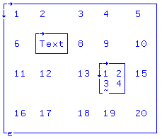
      X[2;2]←⊂"Text"
      X[3;4]←⊂(2 2⍴⍳4)
      X
  1    2  3      4    5
  6 Text  8      9   10

 11   12 13    1 2   15
               3 4

 16   17 18     19   20
|
Element in X[row 2; col 2] is changed (from 7) to a nested vector "Text" using the enclose ⊂ function. Element in X[row 3; col 4], formerly integer 14, now becomes a mini enclosed or ⊂ nested 2x2 matrix of 4 consecutive integers. Since X contains numbers, text and nested elements, it is both a mixed and a nested array. |
Flow control
The user may define custom functions which, like variables, are identified by name rather than by a non-textual symbol. The function header defines whether a custom function is niladic (no arguments), monadic (one right argument) or dyadic (left and right arguments), the local name of the result (to the left of the ← assign arrow), and whether it has any local variables (each separated by semicolon ';').
| Niladic function PI or π(pi) | Monadic function CIRCLEAREA | Dyadic function SEGMENTAREA, with local variables |
|---|---|---|
 ∇ RESULT←PI
   RESULT←○1
 ∇
|
 ∇ AREA←CIRCLEAREA RADIUS
   AREA←PI×RADIUS⋆2
 ∇
|
 ∇ AREA←DEGREES SEGMENTAREA RADIUS ; FRACTION ; CA
   FRACTION←DEGREES÷360
   CA←CIRCLEAREA RADIUS
   AREA←FRACTION×CA
 ∇
|
Whether functions with the same identifier but different adicity are distinct is implementation-defined. If allowed, then a function CURVEAREA could be defined twice to replace both monadic CIRCLEAREA and dyadic SEGMENTAREA above, with the monadic or dyadic function being selected by the context in which it was referenced.
Custom dyadic functions may usually be applied to parameters with the same conventions as built-in functions, i.e. arrays should either have the same number of elements or one of them should have a single element which is extended. There are exceptions to this, for example a function to convert pre-decimal UK currency to dollars would expect to take a parameter with precisely three elements representing pounds, shillings and pence.[10]
Inside a program or a custom function, control may be conditionally transferred to a statement identified by a line number or explicit label; if the target is 0 (zero) this terminates the program or returns to a function's caller. The most common form uses the APL compression function, as in the template (condition)/target which has the effect of evaluating the condition to 0 (false) or 1 (true) and then using that to mask the target (if the condition is false it is ignored, if true it is left alone so control is transferred).
Hence function SEGMENTAREA may be modified to abort (just below), returning zero if the parameters (DEGREES and RADIUS below) are of different sign:
∇ AREA←DEGREES SEGMENTAREA RADIUS ; FRACTION ; CA ; SIGN     ⍝ local variables denoted by semicolon(;)
  FRACTION←DEGREES÷360
  CA←CIRCLEAREA RADIUS        ⍝ this APL code statement calls user function CIRCLEAREA, defined up above.
  SIGN←(×DEGREES)≠×RADIUS     ⍝ << APL logic TEST/determine whether DEGREES and RADIUS do NOT (≠ used) have same SIGN 1-yes different(≠), 0-no(same sign)
  AREA←0                      ⍝ default value of AREA set = zero
  →SIGN/0                     ⍝ branching(here, exiting) occurs when SIGN=1 while SIGN=0 does NOT branch to 0.  Branching to 0 exits function.
  AREA←FRACTION×CA
∇
The above function SEGMENTAREA works as expected if the parameters are scalars or single-element arrays, but not if they are multiple-element arrays since the condition ends up being based on a single element of the SIGN array - on the other hand, the user function could be modified to correctly handle vectorized arguments. Operation can sometimes be unpredictable since APL defines that computers with vector-processing capabilities should parallelise and may reorder array operations as far as possible - therefore, test and debug user functions particularly if they will be used with vector or even matrix arguments. This affects not only explicit application of a custom function to arrays, but also its use anywhere that a dyadic function may reasonably be used such as in generation of a table of results:
        90 180 270 ¯90 ∘.SEGMENTAREA 1 ¯2 4
0 0 0
0 0 0
0 0 0
0 0 0
A more concise way and sometimes better way - to formulate a function is to avoid explicit transfers of control, instead using expressions which evaluate correctly in all or the expected conditions. Sometimes it is correct to let a function fail when one or both input arguments are incorrect - precisely to let user know that one or both arguments used were incorrect. The following is more concise than the above SEGMENTAREA function. The below importantly correctly handles vectorized arguments:
 ∇ AREA←DEGREES SEGMENTAREA RADIUS ; FRACTION ; CA ; SIGN
   FRACTION←DEGREES÷360
   CA←CIRCLEAREA RADIUS
   SIGN←(×DEGREES)≠×RADIUS
   AREA←FRACTION×CA×~SIGN  ⍝ this APL statement is more complex, as a one-liner - but it solves vectorized arguments: a tradeoff - complexity vs. branching
 ∇

        90 180 270 ¯90 ∘.SEGMENTAREA 1 ¯2 4
0.785398163 0           12.5663706
1.57079633  0           25.1327412
2.35619449  0           37.6991118
0           ¯3.14159265 0
Avoiding explicit transfers of control also called branching, if not reviewed or carefully controlled - can promote use of excessively complex "one liners," veritably "misunderstood and complex idioms" and a "write-only" style, which has done little to endear APL to influential commentators such as Edsger Dijkstra.[11] Conversely however APL idioms can be fun, educational and useful - if used with helpful comments ⍝, for example including source and intended meaning/functionality of the idiom(s). Here is an APL idioms list, an IBM APL2 idioms list here[12] and Finnish APL idiom library here.
Miscellaneous
| Name(s) | Symbol | Example | Meaning (of example) | Unicode codepoint |
|---|---|---|---|---|
| High minus[13] | ¯ | ¯3 |
Denotes a negative number | U+00AF ¯ |
| Lamp, Comment | ⍝ | ⍝This is a comment |
Everything to the right of ⍝ denotes a comment | U+235D ⍝ |
| RightArrow, Branch, GoTo | → | →This_Label |
→This_Label sends APL execution to This_Label: | U+2192 → |
| Assign, LeftArrow, Set to | ← | B←A |
B←A sets values and shape of B to match A | U+2190 ← |
Most APL implementations support a number of system variables and functions, usually preceded by the ⎕ (quad) and or ")" (hook=close parenthesis) character. Particularly important and widely implemented is the ⎕IO (Index Origin) variable, since while the original IBM APL based its arrays on 1 some newer variants base them on zero:
| User session with APL interpreter | Description |
|---|---|
        X←⍳12
        X
1 2 3 4 5 6 7 8 9 10 11 12
        ⎕IO
1
        X[1]
1
|
X set = to vector of 12 consecutive integers. Initial index origin ⎕IO value = 1. Therefore, the first position in vector X or X[1] = 1 per vector of iota values {1 2 3 4 5 ...}. |
        ⎕IO←0
        X[1]
2
        X[0]
1
|
Index Origin ⎕IO now changed to 0. Therefore, the 'first index position in vector X changes from 1 to 0. Consequently, X[1] then references or points to 2 from {1 2 3 4 5 ...} and X[0] now references 1. |
        ⎕WA
41226371072
|
Quad WA or ⎕WA, another dynamic system variable, shows how much Work Area remains unused or 41,226 megabytes or about 41 gigabytes of unused/additional total free work area available for the APL workspace/program to process using. If this number gets low or approaches zero - the computer may need more RAM, hard drive space or some combination of the two to increase virtual memory. |
        )VARS
X
|
)VARS a system function in APL,[14] toward bottom of the web page), )VARS shows user variable names existing in the current workspace. |
There are also system functions available to users for saving the current workspace e.g. )SAVE and terminating the APL environment, e.g. )OFF - sometimes called hook commands or functions due to the use of a leading right parenthesis or hook.[15] There is some standardization of these quad and hook functions.
Fonts
The Unicode Basic Multilingual Plane includes the APL symbols in the Miscellaneous Technical block,[16] which are therefore usually rendered accurately from the larger Unicode fonts installed with most modern operating systems. These fonts are rarely designed by typographers familiar with APL glyphs. So, while accurate, the glyphs may look unfamiliar to APL programmers or be difficult to distinguish from one another.
Some Unicode fonts have been designed to display APL well: APLX Upright, APL385 Unicode, and SimPL.
Before Unicode, APL interpreters were supplied with fonts in which APL characters were mapped to less commonly used positions in the ASCII character sets, usually in the upper 128 codepoints. These mappings (and their national variations) were sometimes unique to each APL vendor's interpreter, which made the display of APL programs on the Web, in text files and manuals - frequently problematic.
APL2 Keyboard Functions/Symbols Mapping
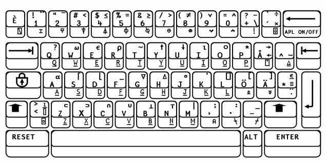
Note the APL On/Off Key - topmost-rightmost key, just below. Also note the keyboard had some 55 unique(68 listed per tables above, including comparative symbols but several symbols appear in both monadic and dyadic tables) APL symbol keys(55 APL functions/operators are listed in IBM's 5110 APL Reference Manual), thus with the use of alt, shift and ctrl keys - it would theoretically have allowed a maximum of some 59(keys) *4(with 2-key pressing) *3(with tri-key pressing, e.g. ctrl-alt-del) or some 472 different maximum key combinations, approaching the 512 EBCDIC character max(256 chars times 2 codes for each keys-combination). Again, in theory the keyboard pictured below would have allowed for about 472 different APL symbols/functions to be keyboard-input, actively used. In practice early versions were only using something roughly equivalent to 55 APL special symbols(excluding letters, numbers, punctuation, etc. keys). Thus early APL was then only using about 11%(55/472) of a symbolic language's at-that-time utilization potential, based on keyboard # keys limits, again excluding numbers, letters, punctuation, etc. In another sense keyboard symbols utilization was closer to 100%, highly efficient, since EBCDIC only allowed 256 distinct chars, and ASCII only 128.
Solving Puzzles
APL has proved to be extremely useful in solving mathematical puzzles, several of which are described below.
Pascal's Triangle
Take Pascal's Triangle, which is a triangular array of numbers in which those at the ends of the rows are 1 and each of the other numbers is the sum of the nearest two numbers in the row just above it (the apex, 1, being at the top). The following is an APL one-liner function to visually depict Pascal's Triangle:
      Pascal←{0~¨⍨a⌽⊃⌽∊¨0,¨¨a∘!¨a←⌽⍳⍵}   ⍝ Create one-line user function called Pascal
      Pascal 7                            ⍝ Run function Pascal for seven rows and show the results below:
                     1
                 1       2
             1       3       3
          1      4       6       4
       1     5       10      10      5
    1     6      15      20      15      6
 1     7     21      35      35      21     7
Prime Numbers, Contra Proof via Factors
Determine the number of prime numbers (prime # is a natural number greater than 1 that has no positive divisors other than 1 and itself) up to some number N. Ken Iverson is credited with the following one-liner APL solution to the problem:
      ⎕CR 'PrimeNumbers'  ⍝ Show APL user-function PrimeNumbers
Primes←PrimeNumbers N     ⍝ Function takes one right arg N (e.g. show prime numbers for 1 ... int N)
Primes←(2=+⌿0=(⍳N)∘.|⍳N)/⍳N  ⍝ The Ken Iverson one-liner
      PrimeNumbers 100    ⍝ Show all prime numbers from 1 to 100
2 3 5 7 11 13 17 19 23 29 31 37 41 43 47 53 59 61 67 71 73 79 83 89 97
      ⍴PrimeNumbers 100
25                       ⍝ There are twenty-five prime numbers in the range up to 100.
Examining the converse or opposite of a mathematical solution is frequently needed (integer factors of a number): Prove for the subset of integers from 1 through 15 that they are non-prime by listing their decomposition factors. What are their non-one factors (#'s divisible by, except 1)?
      ⎕CR 'ProveNonPrime'
Z←ProveNonPrime R
⍝Show all factors of an integer R - except 1 and the number itself,
⍝ i.e. prove Non-Prime. String 'prime' is returned for a Prime integer.
Z←(0=(⍳R)|R)/⍳R  ⍝ Determine all factors for integer R, store into Z
Z←(~(Z∊1,R))/Z   ⍝ Delete 1 and the number as factors for the number from Z.
→(0=⍴Z)/ProveNonPrimeIsPrime               ⍝ If result has zero shape, it has no other factors and is therefore prime
Z←R,(⊂" factors(except 1) "),(⊂Z),⎕TCNL  ⍝ Show the number R, its factors(except 1,itself), and a new line char
→0  ⍝ Done with function if non-prime
ProveNonPrimeIsPrime: Z←R,(⊂" prime"),⎕TCNL  ⍝ function branches here if number was prime

      ProveNonPrime ¨⍳15      ⍝ Prove non primes for each(¨) of the integers from 1 through 15 (iota 15)
    1  prime
    2  prime
    3  prime
    4  factors(except 1)   2
    5  prime
    6  factors(except 1)   2 3
    7  prime
    8  factors(except 1)   2 4
    9  factors(except 1)   3
    10  factors(except 1)   2 5
    11  prime
    12  factors(except 1)   2 3 4 6
    13  prime
    14  factors(except 1)   2 7
    15  factors(except 1)   3 5
Fibonacci Sequence
Generate a Fibonacci Sequence of numbers where each subsequent number in the sequence is the sum of the previous two:
      ⎕CR 'Fibonacci'              ⍝ Display function Fibonacci
FibonacciNum←Fibonacci Nth;IOwas   ⍝ Funct header, funct name=Fibonacci, monadic funct with 1 right hand arg Nth;local var IOwas, and a returned num.
⍝Generate a Fibonacci sequenced number where Nth is the position # of the Fibonacci number in the sequence.  << function description
IOwas←⎕IO ⋄ ⎕IO←0 ⋄ FibonacciNum←↑0 1↓↑+.×/Nth/⊂2 2⍴1 1 1 0 ⋄ ⎕IO←IOwas   ⍝ In order for this function to work correctly ⎕IO must be set to zero.

      Fibonacci¨⍳14    ⍝ This APL statement says: Generate the Fibonacci sequence over each(¨) integer number(iota or ⍳) for the integers 1..14.
0 1 1 2 3 5 8 13 21 34 55 89 144 233   ⍝ Generated sequence, i.e. the Fibonacci sequence of numbers generated by APL's interpreter.
Further reading
- Polivka, Raymond P.; Pakin, Sandra (1975). APL: The Language and Its Usage. Prentice-Hall. ISBN 0-13-038885-8.
- Reiter, Clifford A.; Jones, William R. (1990). APL with a Mathematical Accent (1 ed.). Taylor & Francis. ISBN 978-0534128647. Retrieved 28 January 2015.
- Thompson, Norman D.; Polivka, Raymond P. (2013). APL2 in Depth (Springer Series in Statistics) (Paperback) (Reprint of the original 1st ed.). Springer. ISBN 978-0387942131.
- Gilman, Leonard; Rose, Allen J. (1976). A. P. L.: An Interactive Approach (Paperback) (3rd ed.). ISBN 978-0471093046.
Syntax rules
- Conway's Game Of Life in APL, on YouTube
- APL syntax and semantics[17]
- A future APL: examples and problems[18]
Operators and axis indicator
- The Mathematical Shape of Things to Come "Scientific data sets are becoming more dynamic, requiring new mathematical techniques on par with the invention of calculus." by Jennifer Ouellette, October 4, 2013, Quanta Magazine.[19]
Nested Arrays
- Physicists Probe the Fifth Dimension "The cosmos would make perfect sense ... if it turns out we're living in a 10- or 11-dimensional realm." [20]
- Angiogram analysis in APL: a case study. Angiograms are commonly used to diagnose the occurrence of an arterial occlusion; analysis used 3-dimensional arrays.[21]
- Nested arrays in Plasma Science "Research in the Area of Plasma Science Reported from University of California (Demonstration of Radiation Pulse-Shaping Capabilities Using Nested Conical Wire-Array Z-Pinches)" [22]
APL2 Keyboard Functions/Symbols Mapping
- How to Create an APL or Math Symbols Keyboard Layout[23]
- Technical Keys including APL Keys, Unicodes tables and Symbol representations
- More modern APL keyboard layout information, more on extending APL and its keyboard-symbols-operators.
References
- ↑ Baronet, Dan. "Sharp APL Operators". http://archive.vector.org.uk. Vector - Journal of the British APL Association. Retrieved 13 January 2015. External link in
|website=(help) - ↑ MicroAPL. "Primitive Operators". http://www.microapl.co.uk. MicroAPL. Retrieved 13 January 2015. External link in
|website=(help) - ↑ MicroAPL. "Operators". http://www.microapl.co.uk. MicroAPL. Retrieved 13 January 2015. External link in
|website=(help) - ↑ Progopedia. "APL". http://progopedia.com. Progopedia. Retrieved 13 January 2015. External link in
|website=(help) - ↑ Dyalog. "D-functions and operators loosely grouped into categories". http://dfns.dyalog.com. Dyalog. Retrieved 13 January 2015. External link in
|website=(help) - ↑ IBM. "IBM 5100 APL Reference Manual" (PDF). http://bitsavers.trailing-edge.com. IBM. Retrieved 14 January 2015. External link in
|website=(help) - ↑ Brown, Jim (1978). "In defense of index origin 0". ACM SIGAPL APL Quote Quad. 9 (2): 7 – 7. doi:10.1145/586050.586053. Retrieved 19 January 2015.
- ↑ MicroAPL. "APLX Language Manual" (PDF). http://www.microapl.co.uk. MicroAPL - Version 5 .0 June 2009. p. 22. Retrieved 31 January 2015. External link in
|website=(help) - ↑ Benkard, J. Philip (1992). "Nested Arrays and Operators: Some Issues in Depth". ACM SIGAPL APL Quote Quad. 23 (1): 7–21. doi:10.1145/144045.144065. Retrieved 31 January 2015.
- ↑ Berry, Paul "APL\360 Primer Student Text", IBM Research, Thomas J. Watson Research Center, 1969.
- ↑ https://www.cs.utexas.edu/users/EWD/ewd04xx/EWD498.PDF
- ↑ Cason, Stan. "APL2 Idioms Library". http://www-01.ibm.com. IBM. Retrieved 1 February 2015. External link in
|website=(help) - ↑ APL's "high minus" applies to the single number that follows, while the monadic minus function changes the sign of the entire array to its right.
- ↑ "The Workspace - System Functions"
- ↑ APL language reference
- ↑ Unicode chart "Miscellaneous Technical (including APL)" (PDF).
- ↑ Iverson, Kenneth E. (1983). "APL syntax and semantics". ACM SIGAPL APL Quote Quad. 13 (3): 223–231. doi:10.1145/800062.801221. Retrieved 18 January 2015.
- ↑ Gffer, M. (1989). "A Future APL: Examples and Problems". ACM SIGAPL APL Quote Quad. 19 (4): 158–163. doi:10.1145/75144.75166. Retrieved 18 January 2015.
- ↑ Ouellette, Jennifer. "The Mathematical Shape of Things to Come". https://www.quantamagazine.org. Quanta Magazine. Retrieved 19 January 2015. External link in
|website=(help) - ↑ Boyle, Alan, ed. (2006). "Physicists Probe the Fifth Dimension". http://www.nbcnews.com. NBC News. Retrieved 31 January 2015.
Though these sound like virtually unverifiable claims, physicists are trying to come up with ways to gather evidence to back up or disprove the extradimensional theories...
External link in|website=(help) - ↑ Feldberg, Ian (1990). "Angiogram Analysis in APL: a Case Study". ACM SIGAPL APL Quote Quad. 20 (4): 105. doi:10.1145/97811.97833. Retrieved 31 January 2015.
a 3-dimensional array, where the first dimension represented the image row, the second ...
- ↑ Klir, D. (2013). "Demonstration of Radiation Pulse-Shaping Capabilities Using Nested Conical Wire-Array Z-Pinches". Technology Business Journal. Technology Business Journal / Univ. Andres Bello. 159. ISSN 1945-8401. Retrieved 31 January 2015.
use of these nested conical arrays can potentially provide a valuable tool in X-ray radiation pulse shaping
- ↑ Lee, Xah. "How to Create an APL or Math Symbols Keyboard Layout". http://xahlee.info. Xah Lee. Retrieved 13 January 2015. External link in
|website=(help)
Generic online tutorials
- A Practical Introduction to APL 1 & APL 2 by Graeme Donald Robertson
- APL for PCs, Servers and Tablets - NARS full-featured, no restrictions, free downloadable APL/2 with Nested Arrays by Sudley Place Software
- GNU APL free downloadable interpreter for APL by Jürgen Sauermann
- YouTube APL Tutorials uploaded by Jimin Park, 8 intro/beginner instructional videos.
- SIGAPL Compiled Tutorials List
- Learn APL: An APL Tutorial by MicroAPL
External links
- APL character reference: Page 1, Page 2, Page 3, Page 4
- British APL Association fonts page
- IBM code page 293 aka the APL code page on mainframes
- General information about APL chars on the APL wiki