Affine transformation
In geometry, an affine transformation, affine map[1] or an affinity (from the Latin, affinis, "connected with") is a function between affine spaces which preserves points, straight lines and planes. Also, sets of parallel lines remain parallel after an affine transformation. An affine transformation does not necessarily preserve angles between lines or distances between points, though it does preserve ratios of distances between points lying on a straight line.
Examples of affine transformations include translation, scaling, homothety, similarity transformation, reflection, rotation, shear mapping, and compositions of them in any combination and sequence.
If and are affine spaces, then every affine transformation is of the form , where is a linear transformation on and is a vector in . Unlike a purely linear transformation, an affine map need not preserve the zero point in a linear space. Thus, every linear transformation is affine, but not every affine transformation is linear.


All Euclidean spaces are affine, but there are affine spaces that are non-Euclidean. In affine coordinates, which include Cartesian coordinates in Euclidean spaces, each output coordinate of an affine map is a linear function (in the sense of calculus) of all input coordinates. Another way to deal with affine transformations systematically is to select a point as the origin; then, any affine transformation is equivalent to a linear transformation (of position vectors) followed by a translation.
Mathematical definition
An affine map[1] between two affine spaces is a map on the points that acts linearly on the vectors (that is, the vectors between points of the space). In symbols, determines a linear transformation such that, for any pair of points :


or
- .

We can interpret this definition in a few other ways, as follows.
If an origin is chosen, and denotes its image , then this means that for any vector :


- .

If an origin is also chosen, this can be decomposed as an affine transformation that sends , namely


- ,

followed by the translation by a vector .

The conclusion is that, intuitively, consists of a translation and a linear map.
Alternative definition
Given two affine spaces and , over the same field, a function is an affine map if and only if for every family of weighted points in such that


- ,

we have[2]
- .

In other words, preserves barycenters.
Representation
As shown above, an affine map is the composition of two functions: a translation and a linear map. Ordinary vector algebra uses matrix multiplication to represent linear maps, and vector addition to represent translations. Formally, in the finite-dimensional case, if the linear map is represented as a multiplication by a matrix and the translation as the addition of a vector , an affine map acting on a vector can be represented as


Augmented matrix
Using an augmented matrix and an augmented vector, it is possible to represent both the translation and the linear map using a single matrix multiplication. The technique requires that all vectors are augmented with a "1" at the end, and all matrices are augmented with an extra row of zeros at the bottom, an extra column—the translation vector—to the right, and a "1" in the lower right corner. If is a matrix,
![{\begin{bmatrix}{\vec {y}}\\1\end{bmatrix}}=\left[{\begin{array}{ccc|c}\,&A&&{\vec {b}}\ \\0&\ldots &0&1\end{array}}\right]{\begin{bmatrix}{\vec {x}}\\1\end{bmatrix}}](../I/m/4b3f8dfb50a5d0500891ce899036d73cfd362042.svg)
is equivalent to the following

The above-mentioned augmented matrix is called affine transformation matrix, or projective transformation matrix (as it can also be used to perform projective transformations).
This representation exhibits the set of all invertible affine transformations as the semidirect product of and . This is a group under the operation of composition of functions, called the affine group.


Ordinary matrix-vector multiplication always maps the origin to the origin, and could therefore never represent a translation, in which the origin must necessarily be mapped to some other point. By appending the additional coordinate "1" to every vector, one essentially considers the space to be mapped as a subset of a space with an additional dimension. In that space, the original space occupies the subset in which the additional coordinate is 1. Thus the origin of the original space can be found at . A translation within the original space by means of a linear transformation of the higher-dimensional space is then possible (specifically, a shear transformation). The coordinates in the higher-dimensional space are an example of homogeneous coordinates. If the original space is Euclidean, the higher dimensional space is a real projective space.

The advantage of using homogeneous coordinates is that one can combine any number of affine transformations into one by multiplying the respective matrices. This property is used extensively in computer graphics, computer vision and robotics.
Example augmented matrix
If the vectors are a basis of the domain's projective vector space and if are the corresponding vectors in the codomain vector space then the augmented matrix that achieves this affine transformation


![\left[{\begin{array}{c}{\vec {y}}\\1\end{array}}\right]=M\left[{\begin{array}{c}{\vec {x}}\\1\end{array}}\right]](../I/m/87439de91a378fa59da25f790150e43f7baacf99.svg)
is
- .
![M=\left[{\begin{array}{ccc}{\vec {y}}_{1}&\ldots &{\vec {y}}_{n+1}\\1&\ldots &1\end{array}}\right]\left[{\begin{array}{ccc}{\vec {x}}_{1}&\ldots &{\vec {x}}_{n+1}\\1&\ldots &1\end{array}}\right]^{-1}](../I/m/2dde0e613b3feb9568b081547443e65a0b6e5b3c.svg)
This formulation works irrespective of whether any of the domain, codomain and image vector spaces have the same number of dimensions.
For example, the affine transformation of a vector plane is uniquely determined from the knowledge of where the three vertices of a non-degenerate triangle are mapped to.
Properties
An affine transformation preserves:
- The collinearity relation between points; i.e., points which lie on the same line (called collinear points) continue to be collinear after the transformation.
- Ratios of vectors along a line; i.e., for distinct collinear points the ratio of and is the same as that of and .
- More generally barycenters of weighted collections of points.


An affine transformation is invertible if and only if is invertible. In the matrix representation, the inverse is:
![\left[{\begin{array}{ccc|c}&A^{-1}&&-A^{-1}{\vec {b}}\ \\0&\ldots &0&1\end{array}}\right]](../I/m/99a65ea6867a33379559ae294ae66c1a0269000d.svg)
The invertible affine transformations (of an affine space onto itself) form the affine group, which has the general linear group of degree as subgroup and is itself a subgroup of the general linear group of degree .


The similarity transformations form the subgroup where is a scalar times an orthogonal matrix. For example, if the affine transformation acts on the plane and if the determinant of is 1 or −1 then the transformation is an equiareal mapping. Such transformations form a subgroup called the equi-affine group[3] A transformation that is both equi-affine and a similarity is an isometry of the plane taken with Euclidean distance.
Each of these groups has a subgroup of transformations which preserve orientation: those where the determinant of is positive. In the last case this is in 3D the group of rigid body motions (proper rotations and pure translations).
If there is a fixed point, we can take that as the origin, and the affine transformation reduces to a linear transformation. This may make it easier to classify and understand the transformation. For example, describing a transformation as a rotation by a certain angle with respect to a certain axis may give a clearer idea of the overall behavior of the transformation than describing it as a combination of a translation and a rotation. However, this depends on application and context.
Affine transformation of the plane
Affine transformations in two real dimensions include:
- pure translations,
- scaling in a given direction, with respect to a line in another direction (not necessarily perpendicular), combined with translation that is not purely in the direction of scaling; taking "scaling" in a generalized sense it includes the cases that the scale factor is zero (projection) or negative; the latter includes reflection, and combined with translation it includes glide reflection,
- rotation combined with a homothety and a translation,
- shear mapping combined with a homothety and a translation, or
- squeeze mapping combined with a homothety and a translation.
To visualise the general affine transformation of the Euclidean plane, take labelled parallelograms ABCD and A′B′C′D′. Whatever the choices of points, there is an affine transformation T of the plane taking A to A′, and each vertex similarly. Supposing we exclude the degenerate case where ABCD has zero area, there is a unique such affine transformation T. Drawing out a whole grid of parallelograms based on ABCD, the image T(P) of any point P is determined by noting that T(A) = A′, T applied to the line segment AB is A′B′, T applied to the line segment AC is A′C′, and T respects scalar multiples of vectors based at A. [If A, E, F are collinear then the ratio length(AF)/length(AE) is equal to length(A′F′)/length(A′E′).] Geometrically T transforms the grid based on ABCD to that based in A′B′C′D′.
Affine transformations do not respect lengths or angles; they multiply area by a constant factor
- area of A′B′C′D′ / area of ABCD.
A given T may either be direct (respect orientation), or indirect (reverse orientation), and this may be determined by its effect on signed areas (as defined, for example, by the cross product of vectors).
Examples of affine transformations
Affine transformations over the real numbers
Functions with and constant, are commonplace affine transformations.


Affine transformation over a finite field
The following equation expresses an affine transformation in GF(28):

where is the matrix and is the vector
|
![[M]](../I/m/e5ca74e595b2281c0aef1897ecafa282d1f182e2.svg)


For instance, the affine transformation of the element in big-endian binary notation = in big-endian hexadecimal notation, is calculated as follows:


Thus, .

Affine transformation in plane geometry
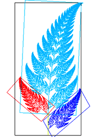
In ℝ2, the transformation shown at left is accomplished using the map given by:

Transforming the three corner points of the original triangle (in red) gives three new points which form the new triangle (in blue). This transformation skews and translates the original triangle.
In fact, all triangles are related to one another by affine transformations. This is also true for all parallelograms, but not for all quadrilaterals.
See also
- The transformation matrix for an affine transformation
- Affine geometry
- 3D projection
- Homography
- Flat (geometry)
- Bent function
Notes
- 1 2 Berger, Marcel (1987), p. 38.
- ↑ Schneider, Philip K. & Eberly, David H. (2003). Geometric Tools for Computer Graphics. Morgan Kaufmann. p. 98. ISBN 978-1-55860-594-7.
- ↑ Oswald Veblen (1918) Projective Geometry, volume 2, pp. 105–7.
References
- Berger, Marcel (1987), Geometry I, Berlin: Springer, ISBN 3-540-11658-3
- Nomizu, Katsumi; Sasaki, S. (1994), Affine Differential Geometry (New ed.), Cambridge University Press, ISBN 978-0-521-44177-3
- Sharpe, R. W. (1997). Differential Geometry: Cartan's Generalization of Klein's Erlangen Program. New York: Springer. ISBN 0-387-94732-9.
External links
- Hazewinkel, Michiel, ed. (2001), "Affine transformation", Encyclopedia of Mathematics, Springer, ISBN 978-1-55608-010-4
- Geometric Operations: Affine Transform, R. Fisher, S. Perkins, A. Walker and E. Wolfart.
- Weisstein, Eric W. "Affine Transformation". MathWorld.
- Affine Transform by Bernard Vuilleumier, Wolfram Demonstrations Project.
- Affine Transformation with MATLAB
| Vector graphics | |
|---|---|
| 2D graphics | |
| 3D graphics | |
| Concepts | |