Big O notation
| Fit approximation | |
|---|---|
|
| |
| Concepts | |
|
Orders of approximation Scale analysis · Big O notation Curve fitting · False precision Significant figures | |
| Other fundamentals | |
|
Approximation · Generalization error Taylor polynomial Scientific modelling | |
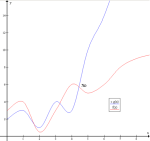
Big O notation is a mathematical notation that describes the limiting behavior of a function when the argument tends towards a particular value or infinity. It is a member of a family of notations invented by Paul Bachmann,[1] Edmund Landau,[2] and others, collectively called Bachmann–Landau notation or asymptotic notation.
In computer science, big O notation is used to classify algorithms by how they respond to changes in input size, such as how the processing time of an algorithm changes as the problem size becomes extremely large.[3] In analytic number theory it is used to estimate the "error committed" while replacing the asymptotic size of an arithmetical function by the value it takes at a large finite argument. A famous example is the problem of estimating the remainder term in the prime number theorem.
Big O notation characterizes functions according to their growth rates: different functions with the same growth rate may be represented using the same O notation.
The letter O is used because the growth rate of a function is also referred to as order of the function. A description of a function in terms of big O notation usually only provides an upper bound on the growth rate of the function. Associated with big O notation are several related notations, using the symbols o, Ω, ω, and Θ, to describe other kinds of bounds on asymptotic growth rates.
Big O notation is also used in many other fields to provide similar estimates.
Formal definition
Let f and g be two functions defined on some subset of the real numbers. One writes

if and only if there is a positive constant M such that for all sufficiently large values of x, the absolute value of f(x) is at most M multiplied by the absolute value of g(x). That is, f(x) = O(g(x)) if and only if there exists a positive real number M and a real number x0 such that
- .

In many contexts, the assumption that we are interested in the growth rate as the variable x goes to infinity is left unstated, and one writes more simply that
- .

The notation can also be used to describe the behavior of f near some real number a (often, a = 0): we say

if and only if there exist positive numbers δ and M such that
- .

If g(x) is non-zero for values of x sufficiently close to a, both of these definitions can be unified using the limit superior:
if and only if
- .

Example
In typical usage, the formal definition of O notation is not used directly; rather, the O notation for a function f is derived by the following simplification rules:
- If f(x) is a sum of several terms, if there is one with largest growth rate, it can be kept, and all others omitted.
- If f(x) is a product of several factors, any constants (terms in the product that do not depend on x) can be omitted.
For example, let f(x) = 6x4 − 2x3 + 5, and suppose we wish to simplify this function, using O notation, to describe its growth rate as x approaches infinity. This function is the sum of three terms: 6x4, −2x3, and 5. Of these three terms, the one with the highest growth rate is the one with the largest exponent as a function of x, namely 6x4. Now one may apply the second rule: 6x4 is a product of 6 and x4 in which the first factor does not depend on x. Omitting this factor results in the simplified form x4. Thus, we say that f(x) is a "big-oh" of (x4). Mathematically, we can write f(x) = O(x4). One may confirm this calculation using the formal definition: let f(x) = 6x4 − 2x3 + 5 and g(x) = x4. Applying the formal definition from above, the statement that f(x) = O(x4) is equivalent to its expansion,

for some suitable choice of x0 and M and for all x > x0. To prove this, let x0 = 1 and M = 13. Then, for all x > x0:

so

Usage
Big O notation has two main areas of application. In mathematics, it is commonly used to describe how closely a finite series approximates a given function, especially in the case of a truncated Taylor series or asymptotic expansion. In computer science, it is useful in the analysis of algorithms. In both applications, the function g(x) appearing within the O(...) is typically chosen to be as simple as possible, omitting constant factors and lower order terms. There are two formally close, but noticeably different, usages of this notation: infinite asymptotics and infinitesimal asymptotics. This distinction is only in application and not in principle, however—the formal definition for the "big O" is the same for both cases, only with different limits for the function argument.
Infinite asymptotics

Big O notation is useful when analyzing algorithms for efficiency. For example, the time (or the number of steps) it takes to complete a problem of size n might be found to be T(n) = 4n2 − 2n + 2. As n grows large, the n2 term will come to dominate, so that all other terms can be neglected—for instance when n = 500, the term 4n2 is 1000 times as large as the 2n term. Ignoring the latter would have negligible effect on the expression's value for most purposes. Further, the coefficients become irrelevant if we compare to any other order of expression, such as an expression containing a term n3 or n4. Even if T(n) = 1,000,000n2, if U(n) = n3, the latter will always exceed the former once n grows larger than 1,000,000 (T(1,000,000) = 1,000,0003= U(1,000,000)). Additionally, the number of steps depends on the details of the machine model on which the algorithm runs, but different types of machines typically vary by only a constant factor in the number of steps needed to execute an algorithm. So the big O notation captures what remains: we write either

or

and say that the algorithm has order of n2 time complexity. Note that "=" is not meant to express "is equal to" in its normal mathematical sense, but rather a more colloquial "is", so the second expression is technically accurate (see the "Equals sign" discussion below) while the first is considered by some as an abuse of notation.[4]
Infinitesimal asymptotics
Big O can also be used to describe the error term in an approximation to a mathematical function. The most significant terms are written explicitly, and then the least-significant terms are summarized in a single big O term. Consider, for example, the exponential series and two expressions of it that are valid when x is small:

The second expression (the one with O(x3)) means the absolute-value of the error ex − (1 + x + x2/2) is at most some constant times |x3| when x is close enough to 0.
Properties
If the function f can be written as a finite sum of other functions, then the fastest growing one determines the order of f(n). For example

In particular, if a function may be bounded by a polynomial in n, then as n tends to infinity, one may disregard lower-order terms of the polynomial. Another thing to notice is the sets O(nc) and O(cn) are very different. If c is greater than one, then the latter grows much faster. A function that grows faster than nc for any c is called superpolynomial. One that grows more slowly than any exponential function of the form cn is called subexponential. An algorithm can require time that is both superpolynomial and subexponential; examples of this include the fastest known algorithms for integer factorization and the function nlog n.
We may ignore any powers of n inside of the logarithms. The set O(log n) is exactly the same as O(log(nc)). The logarithms differ only by a constant factor (since log(nc) = c log n) and thus the big O notation ignores that. Similarly, logs with different constant bases are equivalent. On the other hand, exponentials with different bases are not of the same order. For example, 2n and 3n are not of the same order.
Changing units may or may not affect the order of the resulting algorithm. Changing units is equivalent to multiplying the appropriate variable by a constant wherever it appears. For example, if an algorithm runs in the order of n2, replacing n by cn means the algorithm runs in the order of c2n2, and the big O notation ignores the constant c2. This can be written as c2n2 = O(n2). If, however, an algorithm runs in the order of 2n, replacing n with cn gives 2cn = (2c)n. This is not equivalent to 2n in general. Changing variables may also affect the order of the resulting algorithm. For example, if an algorithm's run time is O(n) when measured in terms of the number n of digits of an input number x, then its run time is O(log x) when measured as a function of the input number x itself, because n = O(log x).
Product


Sum

This implies , which means that is a convex cone.


- If f and g are positive functions,

Multiplication by a constant
- Let k be a constant. Then:
- if k is nonzero.


Multiple variables
Big O (and little o, and Ω...) can also be used with multiple variables. To define Big O formally for multiple variables, suppose and are two functions defined on some subset of . We say


if and only if[5]

Equivalently, the condition that for some can be replaced with the condition that , where denotes the Chebyshev norm. For example, the statement


asserts that there exist constants C and M such that

where g(n,m) is defined by

Note that this definition allows all of the coordinates of to increase to infinity. In particular, the statement


(i.e., ) is quite different from


(i.e., ).

This is not the only generalization of big O to multivariate functions, and in practice, there is some inconsistency in the choice of definition.[6]
Matters of notation
Equals sign
The statement "f(x) is O(g(x))" as defined above is usually written as f(x) = O(g(x)). Some consider this to be an abuse of notation, since the use of the equals sign could be misleading as it suggests a symmetry that this statement does not have. As de Bruijn says, O(x) = O(x2) is true but O(x2) = O(x) is not.[7] Knuth describes such statements as "one-way equalities", since if the sides could be reversed, "we could deduce ridiculous things like n = n2 from the identities n = O(n2) and n2 = O(n2)."[8] For these reasons, it would be more precise to use set notation and write f(x) ∈ O(g(x)), thinking of O(g(x)) as the class of all functions h(x) such that |h(x)| ≤ C|g(x)| for some constant C.[8] However, the use of the equals sign is customary. Knuth pointed out that "mathematicians customarily use the = sign as they use the word 'is' in English: Aristotle is a man, but a man isn't necessarily Aristotle."[9]
Other arithmetic operators
Big O notation can also be used in conjunction with other arithmetic operators in more complicated equations. For example, h(x) + O(f(x)) denotes the collection of functions having the growth of h(x) plus a part whose growth is limited to that of f(x). Thus,

expresses the same as

Example
Suppose an algorithm is being developed to operate on a set of n elements. Its developers are interested in finding a function T(n) that will express how long the algorithm will take to run (in some arbitrary measurement of time) in terms of the number of elements in the input set. The algorithm works by first calling a subroutine to sort the elements in the set and then perform its own operations. The sort has a known time complexity of O(n2), and after the subroutine runs the algorithm must take an additional 55n3 + 2n + 10 steps before it terminates. Thus the overall time complexity of the algorithm can be expressed as T(n) = 55n3 + O(n2). Here the terms 2n+10 are subsumed within the faster-growing O(n2). Again, this usage disregards some of the formal meaning of the "=" symbol, but it does allow one to use the big O notation as a kind of convenient placeholder.
Declaration of variables
Another feature of the notation, although less exceptional, is that function arguments may need to be inferred from the context when several variables are involved. The following two right-hand side big O notations have dramatically different meanings:


The first case states that f(m) exhibits polynomial growth, while the second, assuming m > 1, states that g(n) exhibits exponential growth. To avoid confusion, some authors use the notation

rather than the less explicit

Multiple usages
In more complicated usage, O(...) can appear in different places in an equation, even several times on each side. For example, the following are true for


The meaning of such statements is as follows: for any functions which satisfy each O(...) on the left side, there are some functions satisfying each O(...) on the right side, such that substituting all these functions into the equation makes the two sides equal. For example, the third equation above means: "For any function f(n) = O(1), there is some function g(n) =O(en) such that nf(n) = g(n)." In terms of the "set notation" above, the meaning is that the class of functions represented by the left side is a subset of the class of functions represented by the right side. In this use the "=" is a formal symbol that unlike the usual use of "=" is not a symmetric relation. Thus for example nO(1) = O(en) does not imply the false statement O(en) = nO(1)
Orders of common functions
Here is a list of classes of functions that are commonly encountered when analyzing the running time of an algorithm. In each case, c is a positive constant and n increases without bound. The slower-growing functions are generally listed first.
| Notation | Name | Example |
|---|---|---|
| constant | Determining if a binary number is even or odd; Calculating ; Using a constant-size lookup table | |
| double logarithmic | Number of comparisons spent finding an item using interpolation search in a sorted array of uniformly distributed values | |
| logarithmic | Finding an item in a sorted array with a binary search or a balanced search tree as well as all operations in a Binomial heap | |
| polylogarithmic | Matrix chain ordering can be solved in polylogarithmic time on a Parallel Random Access Machine. | |
| fractional power | Searching in a kd-tree | |
| linear | Finding an item in an unsorted list or in an unsorted array; adding two n-bit integers by ripple carry | |
| n log-star n | Performing triangulation of a simple polygon using Seidel's algorithm, or the union–find algorithm. Note that | |
| linearithmic, loglinear, or quasilinear | Performing a fast Fourier transform; Fastest possible comparison sort; heapsort and merge sort | |
| quadratic | Multiplying two n-digit numbers by a simple algorithm; simple sorting algorithms, such as bubble sort, selection sort and insertion sort; bound on some usually faster sorting algorithms such as including quicksort, Shellsort, and tree sort | |
| polynomial or algebraic | Tree-adjoining grammar parsing; maximum matching for bipartite graphs | |
| L-notation or sub-exponential | Factoring a number using the quadratic sieve or number field sieve | |
| exponential | Finding the (exact) solution to the travelling salesman problem using dynamic programming; determining if two logical statements are equivalent using brute-force search | |
| factorial | Solving the travelling salesman problem via brute-force search; generating all unrestricted permutations of a poset; finding the determinant with Laplace expansion; enumerating all partitions of a set |


![{\displaystyle L_{n}[\alpha ,c]=e^{(c+o(1))(\ln n)^{\alpha }(\ln \ln n)^{1-\alpha }}}](../I/m/40715162d91a34daf9bcfed5f41d8e336417f803.svg)


The statement is sometimes weakened to to derive simpler formulas for asymptotic complexity. For any and , is a subset of for any , so may be considered as a polynomial with some bigger order.


Related asymptotic notations
Big O is the most commonly used asymptotic notation for comparing functions, although in many cases Big O may be replaced with Big Theta Θ for asymptotically tighter bounds. Here, we define some related notations in terms of Big O, progressing up to the family of Bachmann–Landau notations to which Big O notation belongs.
Little-o notation
The informal assertion "f(x) is little-o of g(x)" is formally written
- f(x) = o(g(x)) ,
or in set notation f(x) ∈ o(g(x)). Intuitively, it means that g(x) grows much faster than f(x), or similarly, that the growth of f(x) is nothing compared to that of g(x).
It assumes that f and g are both functions of one variable. Formally, f(n) = o(g(n)) (or f(n) ∈ o(g(n))) as n → ∞ means that for every positive constant ε there exists a constant N such that

Note the difference between the earlier formal definition for the big-O notation, and the present definition of little-o: while the former has to be true for at least one constant M the latter must hold for every positive constant ε, however small.[4] In this way, little-o notation makes a stronger statement than the corresponding big-O notation: every function that is little-o of g is also big-O of g, but not every function that is big-O of g is also little-o of g (for instance g itself is not, unless it is identically zero near ∞).
If g(x) is nonzero, or at least becomes nonzero beyond a certain point, the relation f(x) = o(g(x)) is equivalent to

For example,


Little-o notation is common in mathematics but rarer in computer science. In computer science, the variable (and function value) is most often a natural number. In mathematics, the variable and function values are often real numbers. The following properties (expressed in the more recent, set-theoretical notation) can be useful:
- for
- (and thus the above properties apply with most combinations of o and O).


As with big O notation, the statement "f(x) is o(g(x)) " is usually written as f(x) = o(g(x)), which some consider an abuse of notation.
Big Omega notation
There are two very widespread and incompatible definitions of the statement

where a is some real number, ∞, or −∞, where f and g are real functions defined in a neighbourhood of a, and where g is positive in this neighbourhood.
The first one (chronologically) is used in analytic number theory, and the other one in computational complexity theory. When the two subjects meet, this situation is bound to generate confusion.
The Hardy–Littlewood definition
In 1914 G.H. Hardy and J.E. Littlewood introduced the new symbol ,[10] which is defined as follows:

- .

Thus is the negation of .


In 1916 the same authors introduced the two new symbols and ,[11] thus defined:


- ;

- .

Hence is the negation of , and is the negation of .


Contrary to a later assertion of D.E. Knuth,[12] Edmund Landau did use these three symbols, with the same meanings, in 1924.[13]
These Hardy-Littlewood symbols are prototypes, which after Landau were never used again exactly thus.
- became , and became .


These three symbols , as well as (meaning that and are both satisfied), are now currently used in analytic number theory.[14]


Simple examples
We have

and more precisely

We have

and more precisely

however

The Knuth definition
In 1976 Donald Knuth published a paper to justify his use of the -symbol to describe a stronger property. Knuth wrote: "For all the applications I have seen so far in computer science, a stronger requirement […] is much more appropriate". He defined

with the comment: "Although I have changed Hardy and Littlewood's definition of , I feel justified in doing so because their definition is by no means in wide use, and because there are other ways to say what they want to say in the comparatively rare cases when their definition applies".[12] However, the Hardy–Littlewood definition had been used for at least 25 years.[15]
Family of Bachmann–Landau notations
| Notation | Name | Intuition | Informal definition: for sufficiently large ... | Formal Definition |
|---|---|---|---|---|
| Big O; Big Oh; Big Omicron[12] | is bounded above by (up to constant factor) asymptotically | for some positive k | ||
| Big Omega | Two definitions :
Number theory: is not dominated by asymptotically Complexity theory: is bounded below by asymptotically |
Number theory:
for infinitely many values of n and for some positive k Complexity theory: for some positive k |
Number theory:
Complexity theory: | |
| Big Theta | is bounded both above and below by asymptotically | for some positive k1, k2 |
| |
| Small O; Small Oh | is dominated by asymptotically | , for every fixed positive number | ||
| Small Omega | dominates asymptotically | , for every fixed positive number | ||
| On the order of | is equal to asymptotically |


Aside from the big O notation, the Big Theta Θ and big Omega Ω notations are the two most often used in computer science; the small omega ω notation is occasionally used in computer science.
Aside from the big O notation, the small o, big Omega Ω and notations are the three most often used in number theory; the small omega ω notation is never used in number theory.

Use in computer science
Informally, especially in computer science, the Big O notation often is permitted to be somewhat abused to describe an asymptotic tight bound where using Big Theta Θ notation might be more factually appropriate in a given context. For example, when considering a function T(n) = 73n3 + 22n2 + 58, all of the following are generally acceptable, but tighter bounds (i.e., numbers 2 and 3 below) are usually strongly preferred over looser bounds (i.e., number 1 below).
- T(n) = O(n100)
- T(n) = O(n3)
- T(n) = Θ(n3)
The equivalent English statements are respectively:
- T(n) grows asymptotically no faster than n100
- T(n) grows asymptotically no faster than n3
- T(n) grows asymptotically as fast as n3.
So while all three statements are true, progressively more information is contained in each. In some fields, however, the big O notation (number 2 in the lists above) would be used more commonly than the Big Theta notation (bullets number 3 in the lists above). For example, if T(n) represents the running time of a newly developed algorithm for input size n, the inventors and users of the algorithm might be more inclined to put an upper asymptotic bound on how long it will take to run without making an explicit statement about the lower asymptotic bound.
Other notation
In Introduction to Algorithms, Cormen, Leiserson, Rivest and Stein consider the set of functions g to which some function f belongs when it satisfies

In a correct notation this set can for instance be called O(g), where
- there exist positive constants c and such that for all .[16]


The authors state that the use of equality operator (=) to denote set membership rather than the set membership operator (∈) is an abuse of notation, but that doing so has advantages.[17] Inside an equation or inequality, the use of asymptotic notation stands for an anonymous function in the set O(g), which eliminates lower-order terms, and helps to reduce inessential clutter in equations, for example:[18]

Extensions to the Bachmann–Landau notations
Another notation sometimes used in computer science is Õ (read soft-O): f(n) = Õ(g(n)) is shorthand for f(n) = O(g(n) logk g(n)) for some k. Essentially, it is big O notation, ignoring logarithmic factors because the growth-rate effects of some other super-logarithmic function indicate a growth-rate explosion for large-sized input parameters that is more important to predicting bad run-time performance than the finer-point effects contributed by the logarithmic-growth factor(s). This notation is often used to obviate the "nitpicking" within growth-rates that are stated as too tightly bounded for the matters at hand (since logk n is always o(nε) for any constant k and any ε > 0).
Also the L notation, defined as
is convenient for functions that are between polynomial and exponential in terms of .

Generalizations and related usages
The generalization to functions taking values in any normed vector space is straightforward (replacing absolute values by norms), where f and g need not take their values in the same space. A generalization to functions g taking values in any topological group is also possible. The "limiting process" x→xo can also be generalized by introducing an arbitrary filter base, i.e. to directed nets f and g. The o notation can be used to define derivatives and differentiability in quite general spaces, and also (asymptotical) equivalence of functions,

which is an equivalence relation and a more restrictive notion than the relationship "f is Θ(g)" from above. (It reduces to lim f / g = 1 if f and g are positive real valued functions.) For example, 2x is Θ(x), but 2x − x is not o(x).
History (Bachmann–Landau, Hardy, and Vinogradov notations)
The symbol O was first introduced by number theorist Paul Bachmann in 1894, in the second volume of his book Analytische Zahlentheorie ("analytic number theory"), the first volume of which (not yet containing big O notation) was published in 1892.[1] The number theorist Edmund Landau adopted it, and was thus inspired to introduce in 1909 the notation o;[2] hence both are now called Landau symbols. These notations were used in applied mathematics during the 1950s for asymptotic analysis.[19] The big O was popularized in computer science by Donald Knuth, who re-introduced the related Omega and Theta notations.[12] Knuth also noted that the Omega notation had been introduced by Hardy and Littlewood[10] under a different meaning "≠o" (i.e. "is not an o of"), and proposed the above definition. Hardy and Littlewood's original definition (which was also used in one paper by Landau[13]) is still used in number theory (where Knuth's definition is never used). In fact, Landau also used in 1924, in the paper just mentioned, the symbols ("right") and ("left"), which were introduced in 1918 by Hardy and Littlewood,[11] and which were precursors for the modern symbols ("is not smaller than a small o of") and ("is not larger than a small o of"). Thus the Omega symbols (with their original meanings) are sometimes also referred to as "Landau symbols".
Also, Landau never used the Big Theta and small omega symbols.
Hardy's symbols were (in terms of the modern O notation)
- and


(Hardy however never defined or used the notation , nor , as it has been sometimes reported). It should also be noted that Hardy introduces the symbols and (as well as some other symbols) in his 1910 tract "Orders of Infinity", and makes use of it only in three papers (1910–1913). In his nearly 400 remaining papers and books he consistently uses the Landau symbols O and o.


Hardy's notation is not used anymore. On the other hand, in the 1930s,[20] the Russian number theorist Ivan Matveyevich Vinogradov introduced his notation , which has been increasingly used in number theory instead of the notation. We have


and frequently both notations are used in the same paper.
The big-O originally stands for "order of" ("Ordnung", Bachmann 1894), and is thus a Latin letter. Neither Bachmann nor Landau ever call it "Omicron". The symbol was much later on (1976) viewed by Knuth as a capital omicron,[12] probably in reference to his definition of the symbol Omega. The digit zero should not be used.
See also
- Asymptotic expansion: Approximation of functions generalizing Taylor's formula
- Asymptotically optimal: A phrase frequently used to describe an algorithm that has an upper bound asymptotically within a constant of a lower bound for the problem
- Big O in probability notation: Op,op
- Limit superior and limit inferior: An explanation of some of the limit notation used in this article
- Nachbin's theorem: A precise method of bounding complex analytic functions so that the domain of convergence of integral transforms can be stated
- Orders of approximation
References and Notes
- 1 2 Bachmann, Paul (1894). Analytische Zahlentheorie [Analytic Number Theory] (in German). 2. Leipzig: Teubner.
- 1 2 Landau, Edmund (1909). Handbuch der Lehre von der Verteilung der Primzahlen [Handbook on the theory of the distribution of the primes] (in German). Leipzig: B. G. Teubner. p. 883.
- ↑ Mohr, Austin. "Quantum Computing in Complexity Theory and Theory of Computation" (PDF). p. 2. Retrieved 7 June 2014.
- 1 2 Thomas H. Cormen et al., 2001, Introduction to Algorithms, Second Edition
- ↑ Cormen, Thomas; Leiserson, Charles; Rivest, Ronald; Stein, Clifford (2009). Introduction to Algorithms (Third ed.). MIT. p. 53.
- ↑ Howell, Rodney. "On Asymptotic Notation with Multiple Variables" (PDF). Retrieved 2015-04-23.
- ↑ N. G. de Bruijn (1958). Asymptotic Methods in Analysis. Amsterdam: North-Holland. pp. 5–7. ISBN 978-0-486-64221-5.
- 1 2 3 Graham, Ronald; Knuth, Donald; Patashnik, Oren (1994). Concrete Mathematics (2 ed.). Reading, Massachusetts: Addison–Wesley. p. 446. ISBN 978-0-201-55802-9.
- ↑ Donald Knuth (June–July 1998). "Teach Calculus with Big O" (PDF). Notices of the American Mathematical Society. 45 (6): 687. (Unabridged version)
- 1 2 G. H. Hardy and J. E. Littlewood, "Some problems of Diophantine approximation", Acta Mathematica 37 (1914), p. 225
- 1 2 G. H. Hardy and J. E. Littlewood, « Contribution to the theory of the Riemann zeta-function and the theory of the distribution of primes », Acta Mathematica, vol. 41, 1916.
- 1 2 3 4 5 Donald Knuth. "Big Omicron and big Omega and big Theta", SIGACT News, Apr.-June 1976, 18-24.
- 1 2 E. Landau, "Über die Anzahl der Gitterpunkte in gewissen Bereichen. IV." Nachr. Gesell. Wiss. Gött. Math-phys. Kl. 1924, 137–150.
- ↑ Aleksandar Ivić. The Riemann zeta-function, chapter 9. John Wiley & Sons 1985.
- ↑ E. C. Titchmarsh, The Theory of the Riemann Zeta-Function (Oxford; Clarendon Press, 1951)
- ↑ Thomas H. Cormen; Charles E. Leiserson; Ronald L. Rivest (2009). Introduction to Algorithms (3rd ed.). Cambridge/MA: MIT Press. p. 47. ISBN 978-0262533058.
When we have only an asymptotic upper bound, we use O-notation. For a given function g(n), we denote by O(g(n)) (pronounced “big-oh of g of n” or sometimes just “oh of g of n”) the set of functions O(g(n)) = { f(n) : there exist positive constants c and n0 such that 0 ≤ f(n) ≤ cg(n) for all n ≥ n0}
- ↑ Thomas H. Cormen; Charles E. Leiserson; Ronald L. Rivest (2009). Introduction to Algorithms (3rd ed.). Cambridge/MA: MIT Press. p. 45. ISBN 978-0262533058.
Because θ(g(n)) is a set, we could write "f(n) ∈ θ(g(n))" to indicate that f(n) is a member of θ(g(n)). Instead, we will usually write f(n) = θ(g(n)) to express the same notion. You might be confused because we abuse equality in this way, but we shall see later in this section that doing so has its advantages.
- ↑ Thomas H. Cormen; Charles E. Leiserson; Ronald L. Rivest (2009). Introduction to Algorithms (3rd ed.). Cambridge/MA: MIT Press. p. 49. ISBN 978-0262533058.
When the asymptotic notation stands alone (that is, not within a larger formula) on the right-hand side of an equation (or inequality), as in n = O(n²), we have already defined the equal sign to mean set membership: n ∈ O(n²). In general, however, when asymptotic notation appears in a formula, we interpret it as standing for some anonymous function that we do not care to name. For example, the formula 2n² + 3n + 1 = 2 n² + θ(n) means that 2n² + 3n + 1 = 2 n² + f(n), where f(n) is some function in the set θ(n). In this case, we let f(n) = 3n + 1, which is indeed in θ(n). Using asymptotic notation in this manner can help eliminate inessential detail and clutter in an equation.
- ↑ Erdelyi, A. (1956). Asymptotic Expansions. ISBN 978-0486603186.
- ↑ See for instance "A new estimate for G(n) in Waring's problem" (Russian). Doklady Akademii Nauk SSSR 5, No 5-6 (1934), 249-253. Translated in English in: Selected works / Ivan Matveevič Vinogradov ; prepared by the Steklov Mathematical Institute of the Academy of Sciences of the USSR on the occasion of his 90th birthday. Springer-Verlag, 1985.
Further reading
- Hardy, G. H. (1910). Orders of Infinity: The 'Infinitärcalcül' of Paul du Bois-Reymond. Cambridge University Press.
- Knuth, Donald (1997). "1.2.11: Asymptotic Representations". Fundamental Algorithms. The Art of Computer Programming. 1 (3rd ed.). Addison–Wesley. ISBN 0-201-89683-4.
- Vitányi, Paul; Meertens, Lambert (April 1985). "Big Omega versus the wild functions". ACM SIGACT News. 16 (4): 56–59. doi:10.1145/382242.382835.
- Cormen, Thomas H.; Leiserson, Charles E.; Rivest, Ronald L.; Stein, Clifford (2001). "3.1: Asymptotic notation". Introduction to Algorithms (2nd ed.). MIT Press and McGraw–Hill. ISBN 0-262-03293-7.
- Sipser, Michael (1997). Introduction to the Theory of Computation. PWS Publishing. pp. 226–228. ISBN 0-534-94728-X.
- Avigad, Jeremy; Donnelly, Kevin (2004). Formalizing O notation in Isabelle/HOL (PDF). International Joint Conference on Automated Reasoning. doi:10.1007/978-3-540-25984-8_27.
- Black, Paul E. (11 March 2005). Black, Paul E., ed. "big-O notation". Dictionary of Algorithms and Data Structures. U.S. National Institute of Standards and Technology. Retrieved December 16, 2006.
- Black, Paul E. (17 December 2004). Black, Paul E., ed. "little-o notation". Dictionary of Algorithms and Data Structures. U.S. National Institute of Standards and Technology. Retrieved December 16, 2006.
- Black, Paul E. (17 December 2004). Black, Paul E., ed. "Ω". Dictionary of Algorithms and Data Structures. U.S. National Institute of Standards and Technology. Retrieved December 16, 2006.
- Black, Paul E. (17 December 2004). Black, Paul E., ed. "ω". Dictionary of Algorithms and Data Structures. U.S. National Institute of Standards and Technology. Retrieved December 16, 2006.
- Black, Paul E. (17 December 2004). Black, Paul E., ed. "Θ". Dictionary of Algorithms and Data Structures. U.S. National Institute of Standards and Technology. Retrieved December 16, 2006.
External links
| The Wikibook Data Structures has a page on the topic of: Big-O Notation |
- Growth of sequences — OEIS (Online Encyclopedia of Integer Sequences) Wiki
- Introduction to Asymptotic Notations
- Landau Symbols
- Big-O Notation – What is it good for