Binomial heap

For binomial price trees, see Binomial options pricing model.

In computer science, a binomial heap is a heap similar to a binary heap but also supports quick merging of two heaps. This is achieved by using a special tree structure. It is important as an implementation of the mergeable heap abstract data type (also called meldable heap), which is a priority queue supporting merge operation.

Binomial heap

A binomial heap is implemented as a collection of binomial trees (compare with a binary heap, which has a shape of a single binary tree), which are defined recursively as follows:

• A binomial tree of order 0 is a single node
• A binomial tree of order k has a root node whose children are roots of binomial trees of orders k−1, k−2, ..., 2, 1, 0 (in this order).

Binomial trees of order 0 to 3: Each tree has a root node with subtrees of all lower ordered binomial trees, which have been highlighted. For example, the order 3 binomial tree is connected to an order 2, 1, and 0 (highlighted as blue, green and red respectively) binomial tree.

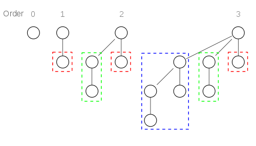
A binomial tree of order k has 2^k nodes, height k.

Because of its unique structure, a binomial tree of order k can be constructed from two trees of order k−1 trivially by attaching one of them as the leftmost child of the root of the other tree. This feature is central to the merge operation of a binomial heap, which is its major advantage over other conventional heaps.

The name comes from the shape: a binomial tree of order $n$ has $\tbinom n d$ nodes at depth $d$. (See Binomial coefficient.)

Structure of a binomial heap

A binomial heap is implemented as a set of binomial trees that satisfy the binomial heap properties:

• Each binomial tree in a heap obeys the minimum-heap property: the key of a node is greater than or equal to the key of its parent.
• There can only be either one or zero binomial trees for each order, including zero order.

The first property ensures that the root of each binomial tree contains the smallest key in the tree, which applies to the entire heap.

The second property implies that a binomial heap with n nodes consists of at most log n + 1 binomial trees. In fact, the number and orders of these trees are uniquely determined by the number of nodes n: each binomial tree corresponds to one digit in the binary representation of number n. For example number 13 is 1101 in binary, $2^3 + 2^2 + 2^0$, and thus a binomial heap with 13 nodes will consist of three binomial trees of orders 3, 2, and 0 (see figure below).

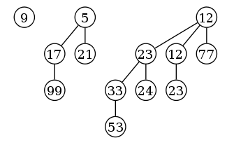
Example of a binomial heap containing 13 nodes with distinct keys.
The heap consists of three binomial trees with orders 0, 2, and 3.

Implementation

Because no operation requires random access to the root nodes of the binomial trees, the roots of the binomial trees can be stored in a linked list, ordered by increasing order of the tree.

Merge

To merge two binomial trees of the same order, first compare the root key. Since 7>3, the black tree on the left(with root node 7) is attached to the grey tree on the right(with root node 3) as a subtree. The result is a tree of order 3.

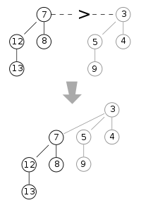
As mentioned above, the simplest and most important operation is the merging of two binomial trees of the same order within a binomial heap. Due to the structure of binomial trees, they can be merged trivially. As their root node is the smallest element within the tree, by comparing the two keys, the smaller of them is the minimum key, and becomes the new root node. Then the other tree becomes a subtree of the combined tree. This operation is basic to the complete merging of two binomial heaps.

function mergeTree(p, q)
    if p.root.key <= q.root.key
        return p.addSubTree(q)
    else
        return q.addSubTree(p)

This shows the merger of two binomial heaps. This is accomplished by merging two binomial trees of the same order one by one. If the resulting merged tree has the same order as one binomial tree in one of the two heaps, then those two are merged again.

The operation of merging two heaps is perhaps the most interesting and can be used as a subroutine in most other operations. The lists of roots of both heaps are traversed simultaneously in a manner similar to that of the merge algorithm.

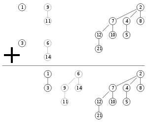
If only one of the heaps contains a tree of order j, this tree is moved to the merged heap. If both heaps contain a tree of order j, the two trees are merged to one tree of order j+1 so that the minimum-heap property is satisfied. Note that it may later be necessary to merge this tree with some other tree of order j+1 present in one of the heaps. In the course of the algorithm, we need to examine at most three trees of any order (two from the two heaps we merge and one composed of two smaller trees).

Because each binomial tree in a binomial heap corresponds to a bit in the binary representation of its size, there is an analogy between the merging of two heaps and the binary addition of the sizes of the two heaps, from right-to-left. Whenever a carry occurs during addition, this corresponds to a merging of two binomial trees during the merge.

Each tree has order at most log n and therefore the running time is O(log n).

function merge(p, q)
    while not (p.end() and q.end())
        tree = mergeTree(p.currentTree(), q.currentTree())
        
        if not heap.currentTree().empty()
            tree = mergeTree(tree, heap.currentTree())
        
        heap.addTree(tree)
        heap.next(); p.next(); q.next()

Insert

Inserting a new element to a heap can be done by simply creating a new heap containing only this element and then merging it with the original heap. Due to the merge, insert takes O(log n) time. However, across a series of n consecutive insertions, insert has an amortized time of O(1) (i.e. constant).

Find minimum

To find the minimum element of the heap, find the minimum among the roots of the binomial trees. This can again be done easily in O(log n) time, as there are just O(log n) trees and hence roots to examine.

By using a pointer to the binomial tree that contains the minimum element, the time for this operation can be reduced to O(1). The pointer must be updated when performing any operation other than Find minimum. This can be done in O(log n) without raising the running time of any operation.

Delete minimum

To delete the minimum element from the heap, first find this element, remove it from its binomial tree, and obtain a list of its subtrees. Then transform this list of subtrees into a separate binomial heap by reordering them from smallest to largest order. Then merge this heap with the original heap. Since each root has at most log n children, creating this new heap is O(log n). Merging heaps is O(log n), so the entire delete minimum operation is O(log n).

function deleteMin(heap)
    min = heap.trees().first()
    for each current in heap.trees()
        if current.root < min.root then min = current
    for each tree in min.subTrees()
        tmp.addTree(tree)
    heap.removeTree(min)
    merge(heap, tmp)

Decrease key

After decreasing the key of an element, it may become smaller than the key of its parent, violating the minimum-heap property. If this is the case, exchange the element with its parent, and possibly also with its grandparent, and so on, until the minimum-heap property is no longer violated. Each binomial tree has height at most log n, so this takes O(log n) time.

Delete

To delete an element from the heap, decrease its key to negative infinity (that is, some value lower than any element in the heap) and then delete the minimum in the heap.

Summary of running times

In the following time complexities^[1] O(f) is an asymptotic upper bound and Θ(f) is an asymptotically tight bound (see Big O notation). Function names assume a min-heap.

Operation	Binary[1]	Binomial[1]	Fibonacci[1]	Pairing[2]	Brodal[3][lower-alpha 1]	Rank-pairing[5]	Strict Fibonacci[6]
find-min	Θ(1)	Θ(log n)	Θ(1)	Θ(1)	Θ(1)	Θ(1)	Θ(1)
delete-min	Θ(log n)	Θ(log n)	O(log n)[lower-alpha 2]	O(log n)[lower-alpha 2]	O(log n)	O(log n)[lower-alpha 2]	O(log n)
insert	O(log n)	Θ(1)[lower-alpha 2]	Θ(1)	Θ(1)	Θ(1)	Θ(1)	Θ(1)
decrease-key	Θ(log n)	Θ(log n)	Θ(1)[lower-alpha 2]	o(log n)[lower-alpha 2][lower-alpha 3]	Θ(1)	Θ(1)[lower-alpha 2]	Θ(1)
merge	Θ(n)	O(log n)[lower-alpha 4]	Θ(1)	Θ(1)	Θ(1)	Θ(1)	Θ(1)

1. Brodal and Okasaki later describe a persistent variant with the same bounds except for decrease-key, which is not supported. Heaps with n elements can be constructed bottom-up in O(n).^[4]
2. Amortized time.
3. Bounded by $\Omega (\log \log n),O(2^{2{\sqrt {\log \log n}}})$^[7][8]
4. n is the size of the larger heap.

Applications

• Discrete event simulation
• Priority queues

See also

• Fibonacci heap
• Soft heap
• Skew binomial heap

References

• Thomas H. Cormen, Charles E. Leiserson, Ronald L. Rivest, and Clifford Stein. Introduction to Algorithms, Second Edition. MIT Press and McGraw-Hill, 2001. ISBN 0-262-03293-7. Chapter 19: Binomial Heaps, pp. 455–475.
• Vuillemin, J. (1978). A data structure for manipulating priority queues. Communications of the ACM 21, 309–314.

External links

• Java applet simulation of binomial heap
• Python implementation of binomial heap
• Two C implementations of binomial heap (a generic one and one optimized for integer keys)
• Haskell implementation of binomial heap
• Common Lisp implementation of binomial heap

1. Cormen, Thomas H.; Leiserson, Charles E.; Rivest, Ronald L. (1990). Introduction to Algorithms (1st ed.). MIT Press and McGraw-Hill. ISBN 0-262-03141-8.
2. Iacono, John (2000), "Improved upper bounds for pairing heaps", Proc. 7th Scandinavian Workshop on Algorithm Theory, Lecture Notes in Computer Science, 1851, Springer-Verlag, pp. 63–77, doi:10.1007/3-540-44985-X_5
3. Brodal, Gerth S. (1996), "Worst-Case Efficient Priority Queues", Proc. 7th Annual ACM-SIAM Symposium on Discrete Algorithms (PDF), pp. 52–58
4. Goodrich, Michael T.; Tamassia, Roberto (2004). "7.3.6. Bottom-Up Heap Construction". Data Structures and Algorithms in Java (3rd ed.). pp. 338–341.
5. Haeupler, Bernhard; Sen, Siddhartha; Tarjan, Robert E. (2009). "Rank-pairing heaps" (PDF). SIAM J. Computing: 1463–1485.
6. Brodal, G. S. L.; Lagogiannis, G.; Tarjan, R. E. (2012). Strict Fibonacci heaps (PDF). Proceedings of the 44th symposium on Theory of Computing - STOC '12. p. 1177. doi:10.1145/2213977.2214082. ISBN 9781450312455.
7. Fredman, Michael Lawrence; Tarjan, Robert E. (1987). "Fibonacci heaps and their uses in improved network optimization algorithms" (PDF). Journal of the Association for Computing Machinery. 34 (3): 596–615. doi:10.1145/28869.28874.
8. Pettie, Seth (2005). "Towards a Final Analysis of Pairing Heaps" (PDF). Max Planck Institut für Informatik.