Bilinear interpolation

In mathematics, bilinear interpolation is an extension of linear interpolation for interpolating functions of two variables (e.g., x and y) on a rectilinear 2D grid.
The key idea is to perform linear interpolation first in one direction, and then again in the other direction. Although each step is linear in the sampled values and in the position, the interpolation as a whole is not linear but rather quadratic in the sample location.
Algorithm
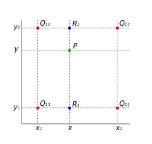
Suppose that we want to find the value of the unknown function f at the point (x, y). It is assumed that we know the value of f at the four points Q11 = (x1, y1), Q12 = (x1, y2), Q21 = (x2, y1), and Q22 = (x2, y2).
We first do linear interpolation in the x-direction. This yields

We proceed by interpolating in the y-direction to obtain the desired estimate:

Note that we will arrive at the same result if the interpolation is done first along the y-direction and then along the x-direction.
Alternative algorithm
An alternative way to write the solution to the interpolation problem is

Where the coefficients are found by solving the linear system

If a solution is preferred in terms of f(Q) then we can write

Where the coefficients are found by solving

Unit Square
If we choose a coordinate system in which the four points where f is known are (0, 0), (0, 1), (1, 0), and (1, 1), then the interpolation formula simplifies to

Or equivalently, in matrix operations:

Nonlinear
Contrary to what the name suggests, the bilinear interpolant is not linear; but it is the product of two linear functions.
Alternatively, the interpolant can be written as

where


In both cases, the number of constants (four) correspond to the number of data points where f is given. The interpolant is linear along lines parallel to either the x or the y direction, equivalently if x or y is set constant. Along any other straight line, the interpolant is quadratic. However, even if the interpolation is not linear in the position (x and y), it is linear in the amplitude, as it is apparent from the equations above: all the coefficient bj, j=1..4, are proportional to the value of the function f(,).
The result of bilinear interpolation is independent of which axis is interpolated first and which second. If we had first performed the linear interpolation in the y-direction and then in the x-direction, the resulting approximation would be the same.
The obvious extension of bilinear interpolation to three dimensions is called trilinear interpolation.
Application in image processing

In computer vision and image processing, bilinear interpolation is one of the basic resampling techniques.
In texture mapping, it is also known as bilinear filtering or bilinear texture mapping, and it can be used to produce a reasonably realistic image. An algorithm is used to map a screen pixel location to a corresponding point on the texture map. A weighted average of the attributes (color, alpha, etc.) of the four surrounding texels is computed and applied to the screen pixel. This process is repeated for each pixel forming the object being textured.[1]
When an image needs to be scaled up, each pixel of the original image needs to be moved in a certain direction based on the scale constant. However, when scaling up an image by a non-integral scale factor, there are pixels (i.e., holes) that are not assigned appropriate pixel values. In this case, those holes should be assigned appropriate RGB or grayscale values so that the output image does not have non-valued pixels.
Bilinear interpolation can be used where perfect image transformation with pixel matching is impossible, so that one can calculate and assign appropriate intensity values to pixels. Unlike other interpolation techniques such as nearest-neighbor interpolation and bicubic interpolation, bilinear interpolation uses only the 4 nearest pixel values which are located in diagonal directions from a given pixel in order to find the appropriate color intensity values of that pixel.
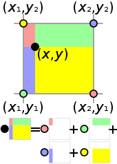
Bilinear interpolation considers the closest 2x2 neighborhood of known pixel values surrounding the unknown pixel's computed location. It then takes a weighted average of these 4 pixels to arrive at its final, interpolated value. The weight on each of the 4 pixel values is based on the computed pixel's distance (in 2D space) from each of the known points.[2]
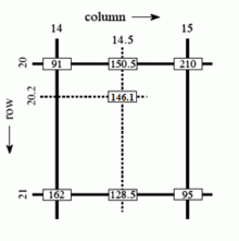
As seen in the example on the right, the intensity value at the pixel computed to be at row 20.2, column 14.5 can be calculated by first linearly interpolating between the values at column 14 and 15 on each rows 20 and 21, giving

and then interpolating linearly between these values, giving

This algorithm reduces some of the visual distortion caused by resizing an image to a non-integral zoom factor, as opposed to nearest-neighbor interpolation, which will make some pixels appear larger than others in the resized image.
See also
- Bicubic interpolation
- Trilinear interpolation
- Spline interpolation
- Lanczos resampling
- Stairstep interpolation
- Barycentric coordinates - for interpolating within a triangle or tetrahedron