Linear interpolation

Given the two red points, the blue line is the linear interpolant between the points, and the value y at x may be found by linear interpolation.

In mathematics, linear interpolation is a method of curve fitting using linear polynomials to construct new data points within the range of a discrete set of known data points.

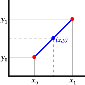
Linear interpolation between two known points

In this geometric visualisation, the value at the green circle multiplied by the distance between the red and blue circles is equal to the sum of the value at the red circle multiplied by the distance between the green and blue circles, and the value at the blue circle multiplied by the distance between the green and red circles.

If the two known points are given by the coordinates $(x_{0},y_{0})$ and $(x_{1},y_{1})$, the linear interpolant is the straight line between these points. For a value x in the interval $(x_{0},x_{1})$, the value y along the straight line is given from the equation

${\frac {y-y_{0}}{x-x_{0}}}={\frac {y_{1}-y_{0}}{x_{1}-x_{0}}}$

which can be derived geometrically from the figure on the right. It is a special case of polynomial interpolation with n = 1.

Solving this equation for y, which is the unknown value at x, gives

${\displaystyle y=y_{0}+(x-x_{0}){\frac {y_{1}-y_{0}}{x_{1}-x_{0}}}}$

which is the formula for linear interpolation in the interval $(x_{0},x_{1})$. Outside this interval, the formula is identical to linear extrapolation.

This formula can also be understood as a weighted average. The weights are inversely related to the distance from the end points to the unknown point; the closer point has more influence than the farther point. Thus, the weights are ${\textstyle {\frac {x-x_{0}}{x_{1}-x_{0}}}}$ and ${\textstyle {\frac {x_{1}-x}{x_{1}-x_{0}}}}$, which are normalized distances between the unknown point and each of the end points. Because these sum to 1,

${\displaystyle y=y_{0}\left(1-{\frac {x-x_{0}}{x_{1}-x_{0}}}\right)+y_{1}\left(1-{\frac {x_{1}-x}{x_{1}-x_{0}}}\right)=y_{0}\left(1-{\frac {x-x_{0}}{x_{1}-x_{0}}}\right)+y_{1}\left({\frac {x-x_{0}}{x_{1}-x_{0}}}\right)}$

which yields the formula for linear interpolation given above.

Interpolation of a data set

Linear interpolation on a data set (red points) consists of pieces of linear interpolants (blue lines).

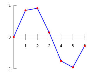
Linear interpolation on a set of data points (x₀, y₀), (x₁, y₁), ..., (x_n, y_n) is defined as the concatenation of linear interpolants between each pair of data points. This results in a continuous curve, with a discontinuous derivative (in general), thus of differentiability class $C^0$.

Linear interpolation as approximation

Linear interpolation is often used to approximate a value of some function f using two known values of that function at other points. The error of this approximation is defined as

$R_T = f(x) - p(x) \,\!$

where p denotes the linear interpolation polynomial defined above

$p(x) = f(x_0) + \frac{f(x_1)-f(x_0)}{x_1-x_0}(x-x_0). \,\!$

It can be proven using Rolle's theorem that if f has a continuous second derivative, the error is bounded by

$|R_T| \leq \frac{(x_1-x_0)^2}{8} \max_{x_0 \leq x \leq x_1} |f''(x)|. \,\!$

As you see, the approximation between two points on a given function gets worse with the second derivative of the function that is approximated. This is intuitively correct as well: the "curvier" the function is, the worse the approximations made with simple linear interpolation.

Applications

Linear interpolation is often used to fill the gaps in a table. Suppose that one has a table listing the population of some country in 1970, 1980, 1990 and 2000, and that one wanted to estimate the population in 1994. Linear interpolation is an easy way to do this.

The basic operation of linear interpolation between two values is commonly used in computer graphics. In that field's jargon it is sometimes called a lerp. The term can be used as a verb or noun for the operation. e.g. "Bresenham's algorithm lerps incrementally between the two endpoints of the line."

Lerp operations are built into the hardware of all modern computer graphics processors. They are often used as building blocks for more complex operations: for example, a bilinear interpolation can be accomplished in three lerps. Because this operation is cheap, it's also a good way to implement accurate lookup tables with quick lookup for smooth functions without having too many table entries.

Extensions

Comparison of linear and bilinear interpolation some 1- and 2-dimensional interpolations. Black and red/yellow/green/blue dots correspond to the interpolated point and neighbouring samples, respectively. Their heights above the ground correspond to their values.

Accuracy

If a C⁰ function is insufficient, for example if the process that has produced the data points is known be smoother than C⁰, it is common to replace linear interpolation with spline interpolation, or even polynomial interpolation in some cases.

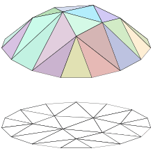
Multivariate

Linear interpolation as described here is for data points in one spatial dimension. For two spatial dimensions, the extension of linear interpolation is called bilinear interpolation, and in three dimensions, trilinear interpolation. Notice, though, that these interpolants are no longer linear functions of the spatial coordinates, rather products of linear functions; this is illustrated by the clearly non-linear example of bilinear interpolation in the figure below. Other extensions of linear interpolation can be applied to other kinds of mesh such as triangular and tetrahedral meshes, including Bézier surfaces. These may be defined as indeed higher-dimensional piecewise linear function (see second figure below).

Example of bilinear interpolation on the unit square with the z-values 0, 1, 1 and 0.5 as indicated. Interpolated values in between represented by colour.

A piecewise linear function in two dimensions (top) and the convex polytopes on which it is linear (bottom).

History

Linear interpolation has been used since antiquity for filling the gaps in tables, often with astronomical data. It is believed that it was used by Babylonian astronomers and mathematicians in Seleucid Mesopotamia (last three centuries BC), and by the Greek astronomer and mathematician, Hipparchus (2nd century BC). A description of linear interpolation can be found in the Almagest (2nd century AD) by Ptolemy.

Programming language support

Many libraries and shading languages have a 'lerp' helper-function, returning an interpolation between two inputs (v0,v1) for a parameter (t) in the closed unit interval [0,1]:

// Imprecise method which does not guarantee v = v1 when t = 1, due to floating-point arithmetic error.
// This form may be used when the hardware has a native Fused Multiply-Add instruction.
float lerp(float v0, float v1, float t) {
  return v0 + t*(v1-v0);
}

// Precise method which guarantees v = v1 when t = 1.
float lerp(float v0, float v1, float t) {
  return (1-t)*v0 + t*v1;
}

This lerp function is commonly used for alpha blending (the parameter 't' is the 'alpha value'), and the formula may be extended to blend multiple components of a vector (such as spatial x,y,z axes, or r,g,b colour components) in parallel.

See also

• Bilinear interpolation
• Spline interpolation
• Polynomial interpolation
• de Casteljau's algorithm
• First-order hold
• Bézier curve

References

• Meijering, Erik (2002), "A chronology of interpolation: from ancient astronomy to modern signal and image processing", Proceedings of the IEEE, 90 (3): 319–342, doi:10.1109/5.993400.

External links

• Linear Interpolation Online Calculation and Visualization Tool
• Equations of the Straight Line at cut-the-knot
• Implementing linear interpolation in Microsoft Excel
• Hazewinkel, Michiel, ed. (2001), "Linear interpolation", Encyclopedia of Mathematics, Springer, ISBN 978-1-55608-010-4
• Hazewinkel, Michiel, ed. (2001), "Finite-increments formula", Encyclopedia of Mathematics, Springer, ISBN 978-1-55608-010-4
• See OrangeOwlSolutions for CUDA implementations of linear interpolation.
• APLJaK Linear Interpolation Calculator one of many calculators available.