Red–black tree
| Red–black tree | ||
|---|---|---|
| Type | Tree | |
| Invented | 1972 | |
| Invented by | Rudolf Bayer | |
| Time complexity in big O notation | ||
| Average | Worst case | |
| Space | O(n) | O(n) |
| Search | O(log n)[1] | O(log n)[1] |
| Insert | O(log n)[1] | O(log n)[1] |
| Delete | O(log n)[1] | O(log n)[1] |
A red–black tree is a kind of self-balancing binary search tree. Each node of the binary tree has an extra bit, and that bit is often interpreted as the color (red or black) of the node. These color bits are used to ensure the tree remains approximately balanced during insertions and deletions.[2]
Balance is preserved by painting each node of the tree with one of two colors (typically called 'red' and 'black') in a way that satisfies certain properties, which collectively constrain how unbalanced the tree can become in the worst case. When the tree is modified, the new tree is subsequently rearranged and repainted to restore the coloring properties. The properties are designed in such a way that this rearranging and recoloring can be performed efficiently.
The balancing of the tree is not perfect, but it is good enough to allow it to guarantee searching in O(log n) time, where n is the total number of elements in the tree. The insertion and deletion operations, along with the tree rearrangement and recoloring, are also performed in O(log n) time.[3]
Tracking the color of each node requires only 1 bit of information per node because there are only two colors. The tree does not contain any other data specific to its being a red–black tree so its memory footprint is almost identical to a classic (uncolored) binary search tree. In many cases the additional bit of information can be stored at no additional memory cost.
History
In 1972 Rudolf Bayer[4] invented a data structure that was a special order-4 case of a B-tree. These trees maintained all paths from root to leaf with the same number of nodes, creating perfectly balanced trees. However, they were not binary search trees. Bayer called them a "symmetric binary B-tree" in his paper and later they became popular as 2-3-4 trees or just 2-4 trees.[5]
In a 1978 paper, "A Dichromatic Framework for Balanced Trees",[6] Leonidas J. Guibas and Robert Sedgewick derived the red-black tree from the symmetric binary B-tree.[7] The color "red" was chosen because it was the best-looking color produced by the color laser printer available to the authors while working at Xerox PARC.[8] Another response from professor Guibas states that it was because of the red and black pens available to them to draw the trees.[9]
In 1993, Arne Andersson introduced the idea of right leaning tree to simplify insert and delete operations.[10]
In 1999, Chris Okasaki showed how to make insert operation purely functional. Its balance function needed to take care of only 4 unbalanced cases and one default balanced case.[11]
The original algorithm used 8 unbalanced cases, but Cormen et al. (2001) reduced that to 6 unbalanced cases.[2] Sedgewick showed that the insert operation can be implemented in just 46 lines of Java code.[12][13] In 2008, Sedgewick proposed the left-leaning red–black tree, leveraging Andersson's idea that simplified algorithms. Sedgewick originally allowed nodes whose two children are red making his trees more like 2-3-4 trees but later this restriction was added making new trees more like 2-3 trees. Sedgewick implemented the insert algorithm in just 33 lines, significantly shortening his original 46 lines of code.[14][15]
Terminology
A red–black tree is a special type of binary tree, used in computer science to organize pieces of comparable data, such as text fragments or numbers.
The leaf nodes of red–black trees do not contain data. These leaves need not be explicit in computer memory—a null child pointer can encode the fact that this child is a leaf—but it simplifies some algorithms for operating on red–black trees if the leaves really are explicit nodes. To save memory, sometimes a single sentinel node performs the role of all leaf nodes; all references from internal nodes to leaf nodes then point to the sentinel node.
Red–black trees, like all binary search trees, allow efficient in-order traversal (that is: in the order Left–Root–Right) of their elements. The search-time results from the traversal from root to leaf, and therefore a balanced tree of n nodes, having the least possible tree height, results in O(log n) search time.
Properties
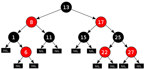
In addition to the requirements imposed on a binary search tree the following must be satisfied by a red–black tree:[16]
- Each node is either red or black.
- The root is black. This rule is sometimes omitted. Since the root can always be changed from red to black, but not necessarily vice versa, this rule has little effect on analysis.
- All leaves (NIL) are black.
- If a node is red, then both its children are black.
- Every path from a given node to any of its descendant NIL nodes contains the same number of black nodes. Some definitions: the number of black nodes from the root to a node is the node's black depth; the uniform number of black nodes in all paths from root to the leaves is called the black-height of the red–black tree.[17]
These constraints enforce a critical property of red–black trees: the path from the root to the farthest leaf is no more than twice as long as the path from the root to the nearest leaf. The result is that the tree is roughly height-balanced. Since operations such as inserting, deleting, and finding values require worst-case time proportional to the height of the tree, this theoretical upper bound on the height allows red–black trees to be efficient in the worst case, unlike ordinary binary search trees.
To see why this is guaranteed, it suffices to consider the effect of properties 4 and 5 together. For a red–black tree T, let B be the number of black nodes in property 5. Let the shortest possible path from the root of T to any leaf consist of B black nodes. Longer possible paths may be constructed by inserting red nodes. However, property 4 makes it impossible to insert more than one consecutive red node. Therefore, ignoring any black NIL leaves, the longest possible path consists of 2*B nodes, alternating black and red (this is the worst case). Counting the black NIL leaves, the longest possible path consists of 2*B-1 nodes.
The shortest possible path has all black nodes, and the longest possible path alternates between red and black nodes. Since all maximal paths have the same number of black nodes, by property 5, this shows that no path is more than twice as long as any other path.
Analogy to B-trees of order 4
.svg.png)
A red–black tree is similar in structure to a B-tree of order[note 1] 4, where each node can contain between 1 and 3 values and (accordingly) between 2 and 4 child pointers. In such a B-tree, each node will contain only one value matching the value in a black node of the red–black tree, with an optional value before and/or after it in the same node, both matching an equivalent red node of the red–black tree.
One way to see this equivalence is to "move up" the red nodes in a graphical representation of the red–black tree, so that they align horizontally with their parent black node, by creating together a horizontal cluster. In the B-tree, or in the modified graphical representation of the red–black tree, all leaf nodes are at the same depth.
The red–black tree is then structurally equivalent to a B-tree of order 4, with a minimum fill factor of 33% of values per cluster with a maximum capacity of 3 values.
This B-tree type is still more general than a red–black tree though, as it allows ambiguity in a red–black tree conversion—multiple red–black trees can be produced from an equivalent B-tree of order 4. If a B-tree cluster contains only 1 value, it is the minimum, black, and has two child pointers. If a cluster contains 3 values, then the central value will be black and each value stored on its sides will be red. If the cluster contains two values, however, either one can become the black node in the red–black tree (and the other one will be red).
So the order-4 B-tree does not maintain which of the values contained in each cluster is the root black tree for the whole cluster and the parent of the other values in the same cluster. Despite this, the operations on red–black trees are more economical in time because you don't have to maintain the vector of values.[18] It may be costly if values are stored directly in each node rather than being stored by reference. B-tree nodes, however, are more economical in space because you don't need to store the color attribute for each node. Instead, you have to know which slot in the cluster vector is used. If values are stored by reference, e.g. objects, null references can be used and so the cluster can be represented by a vector containing 3 slots for value pointers plus 4 slots for child references in the tree. In that case, the B-tree can be more compact in memory, improving data locality.
The same analogy can be made with B-trees with larger orders that can be structurally equivalent to a colored binary tree: you just need more colors. Suppose that you add blue, then the blue–red–black tree defined like red–black trees but with the additional constraint that no two successive nodes in the hierarchy will be blue and all blue nodes will be children of a red node, then it becomes equivalent to a B-tree whose clusters will have at most 7 values in the following colors: blue, red, blue, black, blue, red, blue (For each cluster, there will be at most 1 black node, 2 red nodes, and 4 blue nodes).
For moderate volumes of values, insertions and deletions in a colored binary tree are faster compared to B-trees because colored trees don't attempt to maximize the fill factor of each horizontal cluster of nodes (only the minimum fill factor is guaranteed in colored binary trees, limiting the number of splits or junctions of clusters). B-trees will be faster for performing rotations (because rotations will frequently occur within the same cluster rather than with multiple separate nodes in a colored binary tree). For storing large volumes, however, B-trees will be much faster as they will be more compact by grouping several children in the same cluster where they can be accessed locally.
All optimizations possible in B-trees to increase the average fill factors of clusters are possible in the equivalent multicolored binary tree. Notably, maximizing the average fill factor in a structurally equivalent B-tree is the same as reducing the total height of the multicolored tree, by increasing the number of non-black nodes. The worst case occurs when all nodes in a colored binary tree are black, the best case occurs when only a third of them are black (and the other two thirds are red nodes).
- ↑ Using Knuth's definition of order: the maximum number of children
Applications and related data structures
Red–black trees offer worst-case guarantees for insertion time, deletion time, and search time. Not only does this make them valuable in time-sensitive applications such as real-time applications, but it makes them valuable building blocks in other data structures which provide worst-case guarantees; for example, many data structures used in computational geometry can be based on red–black trees, and the Completely Fair Scheduler used in current Linux kernels uses red–black trees.
The AVL tree is another structure supporting O(log n) search, insertion, and removal. It is more rigidly balanced than red–black trees, leading to slower insertion and removal but faster retrieval. This makes it attractive for data structures that may be built once and loaded without reconstruction, such as language dictionaries (or program dictionaries, such as the opcodes of an assembler or interpreter).
Red–black trees are also particularly valuable in functional programming, where they are one of the most common persistent data structures, used to construct associative arrays and sets which can retain previous versions after mutations. The persistent version of red–black trees requires O(log n) space for each insertion or deletion, in addition to time.
For every 2-4 tree, there are corresponding red–black trees with data elements in the same order. The insertion and deletion operations on 2-4 trees are also equivalent to color-flipping and rotations in red–black trees. This makes 2-4 trees an important tool for understanding the logic behind red–black trees, and this is why many introductory algorithm texts introduce 2-4 trees just before red–black trees, even though 2-4 trees are not often used in practice.
In 2008, Sedgewick introduced a simpler version of the red–black tree called the left-leaning red–black tree[19] by eliminating a previously unspecified degree of freedom in the implementation. The LLRB maintains an additional invariant that all red links must lean left except during inserts and deletes. Red–black trees can be made isometric to either 2-3 trees,[20] or 2-4 trees,[19] for any sequence of operations. The 2-4 tree isometry was described in 1978 by Sedgewick. With 2-4 trees, the isometry is resolved by a "color flip," corresponding to a split, in which the red color of two children nodes leaves the children and moves to the parent node. The tango tree, a type of tree optimized for fast searches, usually uses red–black trees as part of its data structure.
In the version 8 of Java, the Collection HashMap has been modified such that instead of using a LinkedList to store different elements with identical hashcodes, a Red-Black tree is used. This results in the improvement of time complexity of searching such an element from O(n) to O(log n).[21]
Operations
Read-only operations on a red–black tree require no modification from those used for binary search trees, because every red–black tree is a special case of a simple binary search tree. However, the immediate result of an insertion or removal may violate the properties of a red–black tree. Restoring the red–black properties requires a small number (O(log n) or amortized O(1)) of color changes (which are very quick in practice) and no more than three tree rotations (two for insertion). Although insert and delete operations are complicated, their times remain O(log n).
Insertion
Insertion begins by adding the node as any binary search tree insertion does and by coloring it red. Whereas in the binary search tree, we always add a leaf, in the red–black tree, leaves contain no information, so instead we add a red interior node, with two black leaves, in place of an existing black leaf.
What happens next depends on the color of other nearby nodes. The term uncle node will be used to refer to the sibling of a node's parent, as in human family trees. Note that:
- property 3 (all leaves are black) always holds.
- property 4 (both children of every red node are black) is threatened only by adding a red node, repainting a black node red, or a rotation.
- property 5 (all paths from any given node to its leaf nodes contain the same number of black nodes) is threatened only by adding a black node, repainting a red node black (or vice versa), or a rotation.
- Notes
- The label N will be used to denote the current node (colored red). In the diagrams N carries a blue contour. At the beginning, this is the new node being inserted, but the entire procedure may also be applied recursively to other nodes (see case 3). P will denote N's parent node, G will denote N's grandparent, and U will denote N's uncle. In between some cases, the roles and labels of the nodes are exchanged, but in each case, every label continues to represent the same node it represented at the beginning of the case.
- If a node in the right (target) half of a diagram carries a blue contour it will become the current node in the next iteration and there the other nodes will be newly assigned relative to it. Any color shown in the diagram is either assumed in its case or implied by those assumptions.
- A numbered triangle represents a subtree of unspecified depth. A black circle atop a triangle means that black-height of subtree is greater by one compared to subtree without this circle.
There are several cases of red–black tree insertion to handle:
- N is the root node, i.e., first node of red–black tree
- N's parent (P) is black
- N's parent (P) and uncle (U) are red
- N is added to right of left child of grandparent, or N is added to left of right child of grandparent (P is red and U is black)
- N is added to left of left child of grandparent, or N is added to right of right child of grandparent (P is red and U is black)
Each case will be demonstrated with example C code. The uncle and grandparent nodes can be found by these functions:
struct node *grandparent(struct node *n)
{
 if ((n != NULL) && (n->parent != NULL))
  return n->parent->parent;
 else
  return NULL;
}

struct node *uncle(struct node *n)
{
 struct node *g = grandparent(n);
 if (g == NULL)
  return NULL; // No grandparent means no uncle
 if (n->parent == g->left)
  return g->right;
 else
  return g->left;
}
Case 1: The current node N is at the root of the tree. In this case, it is repainted black to satisfy property 2 (the root is black). Since this adds one black node to every path at once, property 5 (all paths from any given node to its leaf nodes contain the same number of black nodes) is not violated.
void insert_case1(struct node *n)
{
 if (n->parent == NULL)
  n->color = BLACK;
 else
  insert_case2(n);
}
Case 2: The current node's parent P is black, so property 4 (both children of every red node are black) is not invalidated. In this case, the tree is still valid. Property 5 (all paths from any given node to its leaf nodes contain the same number of black nodes) is not threatened, because the current node N has two black leaf children, but because N is red, the paths through each of its children have the same number of black nodes as the path through the leaf it replaced, which was black, and so this property remains satisfied.
void insert_case2(struct node *n)
{
 if (n->parent->color == BLACK)
  return; /* Tree is still valid */
 else
  insert_case3(n);
}
- Note: In the following cases it can be assumed that N has a grandparent node G, because its parent P is red, and if it were the root, it would be black. Thus, N also has an uncle node U, although it may be a leaf in cases 4 and 5.
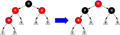 Case 3: If both the parent P and the uncle U are red, then both of them can be repainted black and the grandparent G becomes red (to maintain property 5 (all paths from any given node to its leaf nodes contain the same number of black nodes)). Now, the current red node N has a black parent. Since any path through the parent or uncle must pass through the grandparent, the number of black nodes on these paths has not changed. However, the grandparent G may now violate properties 2 (The root is black) or 4 (Both children of every red node are black) (property 4 possibly being violated since G may have a red parent). To fix this, the entire procedure is recursively performed on G from case 1. Note that this is a tail-recursive call, so it could be rewritten as a loop; since this is the only loop, and any rotations occur after this loop, this proves that a constant number of rotations occur. |
void insert_case3(struct node *n)
{
 struct node *u = uncle(n), *g;

 if ((u != NULL) && (u->color == RED)) {
  n->parent->color = BLACK;
  u->color = BLACK;
  g = grandparent(n);
  g->color = RED;
  insert_case1(g);
 } else {
  insert_case4(n);
 }
}
- Note: In the remaining cases, it is assumed that the parent node P is the left child of its parent. If it is the right child, left and right should be reversed throughout cases 4 and 5. The code samples take care of this.
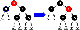
 Case 4: The parent P is red but the uncle U is black; also, the current node N is the right child of P, and P in turn is the left child of its parent G. In this case, a left rotation on P that switches the roles of the current node N and its parent P can be performed; then, the former parent node P is dealt with using case 5 (relabeling N and P) because property 4 (both children of every red node are black) is still violated. The rotation causes some paths (those in the sub-tree labelled "1") to pass through the node N where they did not before. It also causes some paths (those in the sub-tree labelled "3") not to pass through the node P where they did before. However, both of these nodes are red, so property 5 (all paths from any given node to its leaf nodes contain the same number of black nodes) is not violated by the rotation. After this case has been completed, property 4 (both children of every red node are black) is still violated, but now we can resolve this by continuing to case 5. |
void insert_case4(struct node *n)
{
 struct node *g = grandparent(n);

 if ((n == n->parent->right) && (n->parent == g->left)) {
  rotate_left(n->parent);

 /*
 * rotate_left can be the below because of already having *g =  grandparent(n)
 *
 * struct node *saved_p=g->left, *saved_left_n=n->left;
 * g->left=n;
 * n->left=saved_p;
 * saved_p->right=saved_left_n;
 *
 * and modify the parent's nodes properly
 */

  n = n->left;

 } else if ((n == n->parent->left) && (n->parent == g->right)) {
  rotate_right(n->parent);

 /*
 * rotate_right can be the below to take advantage of already having *g =  grandparent(n)
 *
 * struct node *saved_p=g->right, *saved_right_n=n->right;
 * g->right=n;
 * n->right=saved_p;
 * saved_p->left=saved_right_n;
 *
 */

  n = n->right;
 }
 insert_case5(n);
}
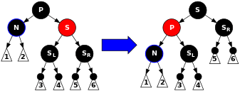
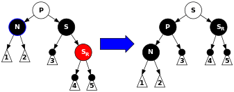
 Case 5: The parent P is red but the uncle U is black, the current node N is the left child of P, and P is the left child of its parent G. In this case, a right rotation on G is performed; the result is a tree where the former parent P is now the parent of both the current node N and the former grandparent G. G is known to be black, since its former child P could not have been red otherwise (without violating property 4). Then, the colors of P and G are switched, and the resulting tree satisfies property 4 (both children of every red node are black). Property 5 (all paths from any given node to its leaf nodes contain the same number of black nodes) also remains satisfied, since all paths that went through any of these three nodes went through G before, and now they all go through P. In each case, this is the only black node of the three. |
void insert_case5(struct node *n)
{
 struct node *g = grandparent(n);

 n->parent->color = BLACK;
 g->color = RED;
 if (n == n->parent->left)
  rotate_right(g);
 else
  rotate_left(g);
}
Note that inserting is actually in-place, since all the calls above use tail recursion.
In the algorithm above, all cases are chained in order, except in insert case 3 where it can recurse to case 1 back to the grandparent node: this is the only case where an iterative implementation will effectively loop. Because the problem of repair is escalated to the next higher level but one, it takes maximally h⁄2 iterations to repair the tree (where h is the height of the tree). Because the probability for escalation decreases exponentially with each iteration the average insertion cost is constant.
Mehlhorn & Sanders (2008) point out: "AVL trees do not support constant amortized update costs", but red-black trees do.[22]
Removal
In a regular binary search tree when deleting a node with two non-leaf children, we find either the maximum element in its left subtree (which is the in-order predecessor) or the minimum element in its right subtree (which is the in-order successor) and move its value into the node being deleted (as shown here). We then delete the node we copied the value from, which must have fewer than two non-leaf children. (Non-leaf children, rather than all children, are specified here because unlike normal binary search trees, red–black trees can have leaf nodes anywhere, so that all nodes are either internal nodes with two children or leaf nodes with, by definition, zero children. In effect, internal nodes having two leaf children in a red–black tree are like the leaf nodes in a regular binary search tree.) Because merely copying a value does not violate any red–black properties, this reduces to the problem of deleting a node with at most one non-leaf child. Once we have solved that problem, the solution applies equally to the case where the node we originally want to delete has at most one non-leaf child as to the case just considered where it has two non-leaf children.
Therefore, for the remainder of this discussion we address the deletion of a node with at most one non-leaf child. We use the label M to denote the node to be deleted; C will denote a selected child of M, which we will also call "its child". If M does have a non-leaf child, call that its child, C; otherwise, choose either leaf as its child, C.
If M is a red node, we simply replace it with its child C, which must be black by property 4. (This can only occur when M has two leaf children, because if the red node M had a black non-leaf child on one side but just a leaf child on the other side, then the count of black nodes on both sides would be different, thus the tree would violate property 5.) All paths through the deleted node will simply pass through one fewer red node, and both the deleted node's parent and child must be black, so property 3 (all leaves are black) and property 4 (both children of every red node are black) still hold.
Another simple case is when M is black and C is red. Simply removing a black node could break Properties 4 (“Both children of every red node are black”) and 5 (“All paths from any given node to its leaf nodes contain the same number of black nodes”), but if we repaint C black, both of these properties are preserved.
The complex case is when both M and C are black. (This can only occur when deleting a black node which has two leaf children, because if the black node M had a black non-leaf child on one side but just a leaf child on the other side, then the count of black nodes on both sides would be different, thus the tree would have been an invalid red–black tree by violation of property 5.) We begin by replacing M with its child C. We will relabel this child C (in its new position) N, and its sibling (its new parent's other child) S. (S was previously the sibling of M.) In the diagrams below, we will also use P for N's new parent (M's old parent), SL for S's left child, and SR for S's right child (S cannot be a leaf because if M and C were black, then P's one subtree which included M counted two black-height and thus P's other subtree which includes S must also count two black-height, which cannot be the case if S is a leaf node).
- Notes
- The label N will be used to denote the current node (colored black). In the diagrams N carries a blue contour. At the beginning, this is the replacement node and a leaf, but the entire procedure may also be applied recursively to other nodes (see case 3). In between some cases, the roles and labels of the nodes are exchanged, but in each case, every label continues to represent the same node it represented at the beginning of the case.
- If a node in the right (target) half of a diagram carries a blue contour it will become the current node in the next iteration and there the other nodes will be newly assigned relative to it. Any color shown in the diagram is either assumed in its case or implied by those assumptions. White represents an arbitrary color (either red or black), but the same in both halves of the diagram.
- A numbered triangle represents a subtree of unspecified depth. A black circle atop a triangle means that black-height of subtree is greater by one compared to subtree without this circle.
We will find the sibling using this function:
struct node *sibling(struct node *n)
{
 if ((n == NULL) || (n->parent == NULL))
  return NULL; // no parent means no sibling
 if (n == n->parent->left)
  return n->parent->right;
 else
  return n->parent->left;
}
- Note: In order that the tree remains well-defined, we need that every null leaf remains a leaf after all transformations (that it will not have any children). If the node we are deleting has a non-leaf (non-null) child N, it is easy to see that the property is satisfied. If, on the other hand, N would be a null leaf, it can be verified from the diagrams (or code) for all the cases that the property is satisfied as well.
We can perform the steps outlined above with the following code, where the function replace_node substitutes child into n's place in the tree. For convenience, code in this section will assume that null leaves are represented by actual node objects rather than NULL (the code in the Insertion section works with either representation).
void delete_one_child(struct node *n)
{
 /*
  * Precondition: n has at most one non-leaf child.
  */
 struct node *child = is_leaf(n->right) ? n->left : n->right;

 replace_node(n, child);
 if (n->color == BLACK) {
  if (child->color == RED)
   child->color = BLACK;
  else
   delete_case1(child);
 }
 free(n);
}
- Note: If N is a null leaf and we do not want to represent null leaves as actual node objects, we can modify the algorithm by first calling delete_case1() on its parent (the node that we delete,
nin the code above) and deleting it afterwards. We do this if the parent is black (red is trivial), so it behaves in the same way as a null leaf (and is sometimes called a 'phantom' leaf). And we can safely delete it at the end asnwill remain a leaf after all operations, as shown above. In addition, the sibling tests in cases 2 and 3 require updating as it is no longer true that the sibling will have children represented as objects.
If both N and its original parent are black, then deleting this original parent causes paths which proceed through N to have one fewer black node than paths that do not. As this violates property 5 (all paths from any given node to its leaf nodes contain the same number of black nodes), the tree must be rebalanced. There are several cases to consider:
Case 1: N is the new root. In this case, we are done. We removed one black node from every path, and the new root is black, so the properties are preserved.
void delete_case1(struct node *n)
{
 if (n->parent != NULL)
  delete_case2(n);
}
- Note: In cases 2, 5, and 6, we assume N is the left child of its parent P. If it is the right child, left and right should be reversed throughout these three cases. Again, the code examples take both cases into account.
 Case 2: S is red. In this case we reverse the colors of P and S, and then rotate left at P, turning S into N's grandparent. Note that P has to be black as it had a red child. The resulting subtree has a path short one black node so we are not done. Now N has a black sibling and a red parent, so we can proceed to step 4, 5, or 6. (Its new sibling is black because it was once the child of the red S.) In later cases, we will relabel N's new sibling as S. |
void delete_case2(struct node *n)
{
 struct node *s = sibling(n);

 if (s->color == RED) {
  n->parent->color = RED;
  s->color = BLACK;
  if (n == n->parent->left)
   rotate_left(n->parent);
  else
   rotate_right(n->parent);
 }
 delete_case3(n);
}
 Case 3: P, S, and S's children are black. In this case, we simply repaint S red. The result is that all paths passing through S, which are precisely those paths not passing through N, have one less black node. Because deleting N's original parent made all paths passing through N have one less black node, this evens things up. However, all paths through P now have one fewer black node than paths that do not pass through P, so property 5 (all paths from any given node to its leaf nodes contain the same number of black nodes) is still violated. To correct this, we perform the rebalancing procedure on P, starting at case 1. |
void delete_case3(struct node *n)
{
 struct node *s = sibling(n);

 if ((n->parent->color == BLACK) &&
     (s->color == BLACK) &&
     (s->left->color == BLACK) &&
     (s->right->color == BLACK)) {
  s->color = RED;
  delete_case1(n->parent);
 } else
  delete_case4(n);
}
 Case 4: S and S's children are black, but P is red. In this case, we simply exchange the colors of S and P. This does not affect the number of black nodes on paths going through S, but it does add one to the number of black nodes on paths going through N, making up for the deleted black node on those paths. |
void delete_case4(struct node *n)
{
 struct node *s = sibling(n);

 if ((n->parent->color == RED) &&
     (s->color == BLACK) &&
     (s->left->color == BLACK) &&
     (s->right->color == BLACK)) {
  s->color = RED;
  n->parent->color = BLACK;
 } else
  delete_case5(n);
}
 Case 5: S is black, S's left child is red, S's right child is black, and N is the left child of its parent. In this case we rotate right at S, so that S's left child becomes S's parent and N's new sibling. We then exchange the colors of S and its new parent. All paths still have the same number of black nodes, but now N has a black sibling whose right child is red, so we fall into case 6. Neither N nor its parent are affected by this transformation. (Again, for case 6, we relabel N's new sibling as S.) |
void delete_case5(struct node *n)
{
 struct node *s = sibling(n);

 if  (s->color == BLACK) { /* this if statement is trivial,
due to case 2 (even though case 2 changed the sibling to a sibling's child,
the sibling's child can't be red, since no red parent can have a red child). */
/* the following statements just force the red to be on the left of the left of the parent,
   or right of the right, so case six will rotate correctly. */
  if ((n == n->parent->left) &&
      (s->right->color == BLACK) &&
      (s->left->color == RED)) { /* this last test is trivial too due to cases 2-4. */
   s->color = RED;
   s->left->color = BLACK;
   rotate_right(s);
  } else if ((n == n->parent->right) &&
             (s->left->color == BLACK) &&
             (s->right->color == RED)) {/* this last test is trivial too due to cases 2-4. */
   s->color = RED;
   s->right->color = BLACK;
   rotate_left(s);
  }
 }
 delete_case6(n);
}
 Case 6: S is black, S's right child is red, and N is the left child of its parent P. In this case we rotate left at P, so that S becomes the parent of P and S's right child. We then exchange the colors of P and S, and make S's right child black. The subtree still has the same color at its root, so Properties 4 (Both children of every red node are black) and 5 (All paths from any given node to its leaf nodes contain the same number of black nodes) are not violated. However, N now has one additional black ancestor: either P has become black, or it was black and S was added as a black grandparent. Thus, the paths passing through N pass through one additional black node. Meanwhile, if a path does not go through N, then there are two possibilities:
Either way, the number of black nodes on these paths does not change. Thus, we have restored Properties 4 (Both children of every red node are black) and 5 (All paths from any given node to its leaf nodes contain the same number of black nodes). The white node in the diagram can be either red or black, but must refer to the same color both before and after the transformation. |
void delete_case6(struct node *n)
{
 struct node *s = sibling(n);

 s->color = n->parent->color;
 n->parent->color = BLACK;

 if (n == n->parent->left) {
  s->right->color = BLACK;
  rotate_left(n->parent);
 } else {
  s->left->color = BLACK;
  rotate_right(n->parent);
 }
}
Again, the function calls all use tail recursion, so the algorithm is in-place.
In the algorithm above, all cases are chained in order, except in delete case 3 where it can recurse to case 1 back to the parent node: this is the only case where an iterative implementation will effectively loop. No more than h loops back to case 1 will occur (where h is the height of the tree). And because the probability for escalation decreases exponentially with each iteration the average removal cost is constant.
Additionally, no tail recursion ever occurs on a child node, so the tail recursion loop can only move from a child back to its successive ancestors. If a rotation occurs in case 2 (which is the only possibility of rotation within the loop of cases 1–3), then the parent of the node N becomes red after the rotation and we will exit the loop. Therefore, at most one rotation will occur within this loop. Since no more than two additional rotations will occur after exiting the loop, at most three rotations occur in total.
Proof of asymptotic bounds
A red black tree which contains n internal nodes has a height of O(log n).
Definitions:
- h(v) = height of subtree rooted at node v
- bh(v) = the number of black nodes from v to any leaf in the subtree, not counting v if it is black - called the black-height
Lemma: A subtree rooted at node v has at least internal nodes.

Proof of Lemma (by induction height):
Basis: h(v) = 0
If v has a height of zero then it must be null, therefore bh(v) = 0. So:

Inductive Step: v such that h(v) = k, has at least internal nodes implies that such that h() = k+1 has at least internal nodes.


Since has h() > 0 it is an internal node. As such it has two children each of which have a black-height of either bh() or bh()-1 (depending on whether the child is red or black, respectively). By the inductive hypothesis each child has at least internal nodes, so has at least:


internal nodes.
Using this lemma we can now show that the height of the tree is logarithmic. Since at least half of the nodes on any path from the root to a leaf are black (property 4 of a red–black tree), the black-height of the root is at least h(root)/2. By the lemma we get:

Therefore, the height of the root is O(log n).
Parallel algorithms
Parallel algorithms for constructing red–black trees from sorted lists of items can run in constant time or O(log log n) time, depending on the computer model, if the number of processors available is asymptotically proportional to the number n of items where n→∞. Fast search, insertion, and deletion parallel algorithms are also known.[23]
Popular Culture
A red-black-tree was referenced correctly in an episode of Missing (Canadian TV series)[24] as noted by Robert Sedgewick in one of his lectures:[25]
Jess: " It was the red door again.
"
Pollock: " I thought the red door was the storage container.
"
Jess: " But it wasn't red anymore, it was black.
"
Antonio: " So red turning to black means what?
"
Pollock: " Budget deficits, red ink, black ink.
"
Antonio: " It could be from a binary search tree. The red-black tree tracks every simple path from a node to a descendant leaf that has the same number of black nodes.
"
Jess: " Does that help you with the ladies?
"
See also
- List of data structures
- Tree data structure
- Tree rotation
- AA tree, a variation of the red-black tree
- AVL tree
- B-tree (2-3 tree, 2-3-4 tree, B+ tree, B*-tree, UB-tree)
- Scapegoat tree
- Splay tree
- T-tree
- WAVL tree
References
- 1 2 3 4 5 6 James Paton. "Red-Black Trees".
- 1 2 Cormen, Thomas H.; Leiserson, Charles E.; Rivest, Ronald L.; Stein, Clifford (2001). "Red–Black Trees". Introduction to Algorithms (second ed.). MIT Press. pp. 273–301. ISBN 0-262-03293-7.
- ↑ John Morris. "Red–Black Trees".
- ↑ Rudolf Bayer (1972). "Symmetric binary B-Trees: Data structure and maintenance algorithms". Acta Informatica. 1 (4): 290–306. doi:10.1007/BF00289509.
- ↑ Drozdek, Adam. Data Structures and Algorithms in Java (2 ed.). Sams Publishing. p. 323. ISBN 0534376681.
- ↑ Leonidas J. Guibas and Robert Sedgewick (1978). "A Dichromatic Framework for Balanced Trees". Proceedings of the 19th Annual Symposium on Foundations of Computer Science. pp. 8–21. doi:10.1109/SFCS.1978.3.
- ↑ "Red Black Trees". eternallyconfuzzled.com. Retrieved 2015-09-02.
- ↑ Robert Sedgewick (2012). Red-Black BSTs. Coursera.
A lot of people ask why did we use the name red–black. Well, we invented this data structure, this way of looking at balanced trees, at Xerox PARC which was the home of the personal computer and many other innovations that we live with today entering[sic] graphic user interfaces, ethernet and object-oriented programmings[sic] and many other things. But one of the things that was invented there was laser printing and we were very excited to have nearby color laser printer that could print things out in color and out of the colors the red looked the best. So, that’s why we picked the color red to distinguish red links, the types of links, in three nodes. So, that’s an answer to the question for people that have been asking.
- ↑ "Where does the term "Red/Black Tree" come from?". programmers.stackexchange.com. Retrieved 2015-09-02.
- ↑ Andersson, Arne (1993-08-11). Dehne, Frank; Sack, Jörg-Rüdiger; Santoro, Nicola; Whitesides, Sue, eds. "Balanced search trees made simple" (PDF). Algorithms and Data Structures (Proceedings). Lecture Notes in Computer Science. Springer-Verlag Berlin Heidelberg. 709: 60–71. doi:10.1007/3-540-57155-8_236. ISBN 978-3-540-57155-1. Archived from the original on 2000-03-17.
- ↑ Okasaki, Chris (1999-01-01). "Red-black trees in a functional setting" (PS). Journal of Functional Programming. 9 (4): 471–477. doi:10.1017/S0956796899003494. ISSN 1469-7653.
- ↑ Sedgewick, Robert (1983). Algorithms (1st ed.). Addison-Wesley. ISBN 0-201-06672-6.
- ↑ RedBlackBST code in Java
- ↑ Sedgewick, Robert (2008). "Left-leaning Red-Black Trees" (PDF).
- ↑
- Sedgewick, Robert; Wayne, Kevin (2011). Algorithms (4th ed.). Addison-Wesley Professional. ISBN 978-0-321-57351-3.
- ↑ Cormen, Thomas; Leiserson, Charles; Rivest, Ronald; Stein, Clifford (2009). "13". Introduction to Algorithms (3rd ed.). MIT Press. pp. 308–309. ISBN 978-0-262-03384-8.
- ↑ Mehlhorn, Kurt; Sanders, Peter (2008). Algorithms and Data Structures: The Basic Toolbox (PDF). Springer, Berlin/Heidelberg. pp. 154–165. doi:10.1007/978-3-540-77978-0. ISBN 978-3-540-77977-3. p. 155.
- ↑ Sedgewick, Robert (1998). Algorithms in C++. Addison-Wesley Professional. pp. 565–575. ISBN 978-0201350883.
- 1 2 http://www.cs.princeton.edu/~rs/talks/LLRB/RedBlack.pdf
- ↑ http://www.cs.princeton.edu/courses/archive/fall08/cos226/lectures/10BalancedTrees-2x2.pdf
- ↑ "How does a HashMap work in JAVA". coding-geek.com.
- ↑ Mehlhorn & Sanders 2008, pp. 165, 158
- ↑ Park, Heejin; Park, Kunsoo (2001). "Parallel algorithms for red–black trees". Theoretical computer science. Elsevier. 262 (1–2): 415–435. doi:10.1016/S0304-3975(00)00287-5.
Our parallel algorithm for constructing a red–black tree from a sorted list of n items runs in O(1) time with n processors on the CRCW PRAM and runs in O(log log n) time with n / log log n processors on the EREW PRAM.
- ↑ Missing (Canadian TV series). A, W Network (Canada); Lifetime (United States).
- ↑ Robert Sedgewick (2012). B-Trees. Coursera. 10:07 minutes in.
So not only is there some excitement in that dialogue but it's also technically correct which you don't often find with math in popular culture of computer science. A red black tree tracks every simple path from a node to a descendant leaf with the same number of black nodes they got that right.
Further reading
- Mathworld: Red–Black Tree
- San Diego State University: CS 660: Red–Black tree notes, by Roger Whitney
- Pfaff, Ben (June 2004). "Performance Analysis of BSTs in System Software" (PDF). Stanford University.
External links
- A complete and working implementation in C
- Red–Black Tree Demonstration
- OCW MIT Lecture by Prof. Erik Demaine on Red Black Trees -
- Binary Search Tree Insertion Visualization on YouTube – Visualization of random and pre-sorted data insertions, in elementary binary search trees, and left-leaning red–black trees
- An intrusive red-black tree written in C++
- Red-black BSTs in 3.3 Balanced Search Trees
- Red–black BST Demo