Blind deconvolution
In electrical engineering and applied mathematics, blind deconvolution is deconvolution without explicit knowledge of the impulse response function used in the convolution. In microscopy the term is used to describe deconvolution without knowledge of the microscopes point spread function. This is usually achieved by making appropriate assumptions of the input to estimate the impulse response by analyzing the output.
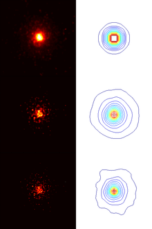
In image processing
In image processing, blind deconvolution is a deconvolution technique that permits recovery of the target scene from a single or set of "blurred" images in the presence of a poorly determined or unknown point spread function (PSF). [2] Regular linear and non-linear deconvolution techniques utilize a known PSF. For blind deconvolution, the PSF is estimated from the image or image set, allowing the deconvolution to be performed. Researchers have been studying blind deconvolution methods for several decades, and have approached the problem from different directions.
Blind deconvolution can be performed iteratively, whereby each iteration improves the estimation of the PSF and the scene, or non-iteratively, where one application of the algorithm, based on exterior information, extracts the PSF. Iterative methods include maximum a posteriori estimation and expectation-maximization algorithms. A good estimate of the PSF is helpful for quicker convergence but not necessary.
Examples of non-iterative techniques include SeDDaRA,[3] the cepstrum transform and APEX. The cepstrum transform and APEX methods assume that the PSF has a specific shape, and one must estimate the width of the shape. For SeDDaRA, the information about the scene is provided in the form of a reference image. The algorithm estimates the PSF by comparing the spatial frequency information in the blurred image to that of the target image.
In signal processing
Seismic data
In the case of deconvolution of seismic data, the original unknown signal is made of spikes hence is possible to characterize with sparsity constraints[4] or regularizations such as l1 norm/l2 norm norm ratios,[5] suggested by W. C. Gray in 1978.[6]
Audio deconvolution
Audio deconvolution (often referred to as dereverberation) is a reverberation reduction in audio mixtures. It is part of audio processing of recordings in ill-posed cases such as the cocktail party effect. One possibility is to use ICA.[7]
In general
Suppose we have a signal transmitted through a channel. The channel can usually be modeled as a linear shift-invariant system, so the receptor receives a convolution of the original signal with the impulse response of the channel. If we want to reverse the effect of the channel, to obtain the original signal, we must process the received signal by a second linear system, inverting the response of the channel. This system is called an equalizer.
If we are given the original signal, we can use a supervising technique, such as finding a Wiener filter, but without it, we can still explore what we do know about it to attempt its recovery. For example, we can filter the received signal to obtain the desired spectral power density. This is what happens, for example, when the original signal is known to have no auto correlation, and we "whiten" the received signal.
Whitening usually leaves some phase distortion in the results. Most blind deconvolution techniques use higher-order statistics of the signals, and permit the correction of such phase distortions. We can optimize the equalizer to obtain a signal with a PSF approximating what we know about the original PSF.
High-order statistics
Blind deconvolution algorithms often make use of high-order statistics, with moments higher than two. This can be implicit or explicit.[8]
See also
- Channel model
- Inverse problem
- Regularization (mathematics)
- Blind equalization
- Maximum a posteriori estimation
- Maximum likelihood
External links
References
- ↑ P. Barmby; D. E. McLaughlin; et al. (2007). "Structural Parameters for Globular Clusters in M31 and Generalizations for the Fundamental Plane" (PDF). The Astronomical Journal. 133 (6): 2764–2786. arXiv:0704.2057
 . Bibcode:2007AJ....133.2764B. doi:10.1086/516777.
- ↑ E. Lam; J.W. Goodman (2000). "Iterative statistical approach to blind image deconvolution". Journal of the Optical Society of America A. 17 (7): 1177–1184. Bibcode:2000JOSAA..17.1177L. doi:10.1364/JOSAA.17.001177.
- ↑ Caron, James N.; Namazi, Nader M.; Rollins, Chris J. (2002-11-11). "Noniterative blind data restoration by use of an extracted filter function". www.osapublishing.org. doi:10.1364/AO.41.006884. Retrieved 2016-03-21.
- ↑ Broadhead, Michael (2010). "Sparse seismic deconvolution by method of orthogonal matching pursuit".
- ↑ A. Repetti; M. Q. Pham; L. Duval; E. Chouzenoux; J.-C. Pesquet (2015). "Euclid in a Taxicab: Sparse Blind Deconvolution with Smoothed l1/l2 Regularization". IEEE Signal Processing Letters: 539–543. arXiv:1407.5465.
- ↑ W. C. Gray (1978). "Variable norm deconvolution" (PDF).
- ↑ Koldovsky, Zbynek & Tichavsky, Petr (2007). "Time-domain blind audio source separation using advanced ICA methods": 846–849,.
- ↑ Cardoso, J-F (1991). "Super-symmetric decomposition of the fourth-order cumulant tensor. Blind identification of more sources than sensors" (PDF). IEEE: 3109–3112.