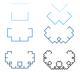
Lévy C curve

In mathematics, the Lévy C curve is a self-similar fractal that was first described and whose differentiability properties were analysed by Ernesto Cesàro in 1906 and Georg Faber in 1910, but now bears the name of French mathematician Paul Lévy, who was the first to describe its self-similarity properties, as well as to provide a geometrical construction showing it as a representative curve in the same class as the Koch curve. It is a special case of a period-doubling curve, a de Rham curve.

L-system construction

First eight stages in the construction of a Lévy C curve

Lévy C curve (from a L-system, after the first 12 stages)

If using a Lindenmayer system then the construction of the C curve starts with a straight line. An isosceles triangle with angles of 45°, 90° and 45° is built using this line as its hypotenuse. The original line is then replaced by the other two sides of this triangle.

At the second stage, the two new lines each form the base for another right-angled isosceles triangle, and are replaced by the other two sides of their respective triangle. So, after two stages, the curve takes the appearance of three sides of a rectangle with the same length as the original line, but only half as wide.

At each subsequent stage, each straight line segment in the curve is replaced by the other two sides of a right-angled isosceles triangle built on it. After n stages the curve consists of 2ⁿ line segments, each of which is smaller than the original line by a factor of 2^n/2.

This L-system can be described as follows:

Variables:	F
Constants:	+ −
Start:	F
Rules:	F → +F−−F+

where "F" means "draw forward", "+" means "turn clockwise 45°", and "−" means "turn anticlockwise 45°".

The fractal curve that is the limit of this "infinite" process is the Lévy C curve. It takes its name from its resemblance to a highly ornamented version of the letter "C". The curve resembles the finer details of the Pythagoras tree.

The Hausdorff dimension of the C curve equals 2 (it contains open sets), whereas the boundary has dimension about 1.9340 .

Variations

The standard C curve is built using 45° isosceles triangles. Variations of the C curve can be constructed by using isosceles triangles with angles other than 45°. As long as the angle is less than 60°, the new lines introduced at each stage are each shorter than the lines that they replace, so the construction process tends towards a limit curve. Angles less than 45° produce a fractal that is less tightly "curled".

IFS construction

Lévy C curve (from IFS, infinite levels)

If using an iterated function system (IFS, or the chaos game IFS-method actually), then the construction of the C curve is a bit easier. It will need a set of two "rules" which are: Two points in a plane (the translators), each associated with a scale factor of 1/√2. The first rule is a rotation of 45° and the second −45°. This set will iterate a point [x, y] from randomly choosing any of the two rules and use the parameters associated with the rule to scale/rotate and translate the point using a 2D-transform function.

Put into formulae:

$f_{1}(z)={\frac {(1-i)z}{2}}$

$f_{2}(z)=1+{\frac {(1+i)(z-1)}{2}}$

from the initial set of points $S_{0}=\{0,1\}$.

Sample Implementation of Levy C Curve

// Java Sample Implementation of Levy C Curve

import java.awt.Color;
import java.awt.Graphics;
import java.awt.Graphics2D;
import javax.swing.JFrame;
import javax.swing.JPanel;
import java.util.concurrent.ThreadLocalRandom;

public class C_curve extends JPanel {

    public float x, y, len, alpha_angle;
    public int iteration_n;

    public void paint(Graphics g) {
        Graphics2D g2d = (Graphics2D) g;
        c_curve(x, y, len, alpha_angle, iteration_n, g2d);
    }

    public void c_curve(double x, double y, double len, double alpha_angle, int iteration_n, Graphics2D g) {
        double fx = x; 
        double fy = y;
        double length = len;
        double alpha = alpha_angle;
        int it_n = iteration_n;
        if (it_n > 0) {
            length = (length / Math.sqrt(2));
            c_curve(fx, fy, length, (alpha + 45), (it_n - 1), g); // Recursive Call
            fx = (fx + (length * Math.cos(Math.toRadians(alpha + 45))));
            fy = (fy + (length * Math.sin(Math.toRadians(alpha + 45))));
            c_curve(fx, fy, length, (alpha - 45), (it_n - 1), g); // Recursive Call
        } else {
            Color[] A = {Color.RED, Color.ORANGE, Color.BLUE, Color.DARK_GRAY};
            g.setColor(A[ThreadLocalRandom.current().nextInt(0, A.length)]); //For Choosing Different Color Values
            g.drawLine((int) fx, (int) fy, (int) (fx + (length * Math.cos(Math.toRadians(alpha)))), (int) (fy + (length * Math.sin(Math.toRadians(alpha)))));
        }
    }

    public static void main(String[] args) {
        C_curve points = new C_curve();
        points.x = 200; // Stating x value
        points.y = 100; // Stating y value
        points.len = 150; // Stating length value
        points.alpha_angle = 90; // Stating angle value
        points.iteration_n = 15; // Stating iteration value

        JFrame frame = new JFrame("Points");
        frame.setDefaultCloseOperation(JFrame.EXIT_ON_CLOSE);
        frame.add(points);
        frame.setSize(500, 500);
        frame.setLocationRelativeTo(null);
        frame.setVisible(true);

    }
}

See also

• Dragon curve
• Pythagoras tree (fractal)

References

• Paul Lévy, Plane or Space Curves and Surfaces Consisting of Parts Similar to the Whole (1938), reprinted in Classics on Fractals Gerald A. Edgar ed. (1993) Addison-Wesley Publishing ISBN 0-201-58701-7.
• E. Cesaro, Fonctions continues sans dérivée, Archiv der Math. und Phys. 10 (1906) pp 57–63.
• G. Faber, Über stetige Funktionen II, Math Annalen, 69 (1910) pp 372–443.
• S. Bailey, T. Kim, R. S. Strichartz, Inside the Lévy dragon, American Mathematical Monthly 109(8) (2002) pp 689–703