Dynamic light scattering
Dynamic light scattering (DLS) is a technique in physics that can be used to determine the size distribution profile of small particles in suspension or polymers in solution.[1] In the scope of DLS, temporal fluctuations are usually analyzed by means of the intensity or photon auto-correlation function (also known as photon correlation spectroscopy or quasi-elastic light scattering). In the time domain analysis, the autocorrelation function (ACF) usually decays starting from zero delay time, and faster dynamics due to smaller particles lead to faster decorrelation of scattered intensity trace. It has been shown that the intensity ACF is the Fourier transformation of the power spectrum, and therefore the DLS measurements can be equally well performed in the spectral domain.[2][3] DLS can also be used to probe the behavior of complex fluids such as concentrated polymer solutions.
Setup
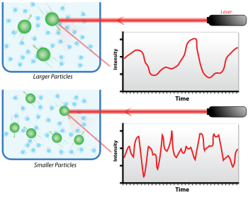
A monochromatic light source, usually a laser, is shot through a polarizer and into a sample. The scattered light then goes through a second polarizer where it is collected by a photomultiplier and the resulting image is projected onto a screen. This is known as a speckle pattern (Figure 1).[4]
All of the molecules in the solution are being hit with the light and all of the molecules diffract the light in all directions. The diffracted light from all of the molecules can either interfere constructively (light regions) or destructively (dark regions). This process is repeated at short time intervals and the resulting set of speckle patterns are analyzed by an autocorrelator that compares the intensity of light at each spot over time. The polarizers can be set up in two geometrical configurations. One is a vertical/vertical (VV) geometry, where the second polarizer allows light through that is in the same direction as the primary polarizer. In vertical/horizontal (VH) geometry the second polarizer allows light not in same direction as the incident light.
Description
When light hits small particles, the light scatters in all directions (Rayleigh scattering) as long as the particles are small compared to the wavelength (below 250 nm). Even if the light source is a laser, and thus is monochromatic and coherent, the scattering intensity fluctuates over time. This fluctuation is due to small molecules in solutions are undergoing Brownian motion, and so the distance between the scatterers in the solution is constantly changing with time. This scattered light then undergoes either constructive or destructive interference by the surrounding particles, and within this intensity fluctuation, information is contained about the time scale of movement of the scatterers. Sample preparation either by filtration or centrifugation is critical to remove dust and artifacts from the solution.
The dynamic information of the particles is derived from an autocorrelation of the intensity trace recorded during the experiment. The second order autocorrelation curve is generated from the intensity trace as follows:

where g2(q;τ) is the autocorrelation function at a particular wave vector, q, and delay time, τ, and I is the intensity. The angular brackets <> denote the expected value operator, which in some texts is denoted by a capital E.
At short time delays, the correlation is high because the particles do not have a chance to move to a great extent from the initial state that they were in. The two signals are thus essentially unchanged when compared after only a very short time interval. As the time delays become longer, the correlation decays exponentially, meaning that, after a long time period has elapsed, there is no correlation between the scattered intensity of the initial and final states. This exponential decay is related to the motion of the particles, specifically to the diffusion coefficient. To fit the decay (i.e., the autocorrelation function), numerical methods are used, based on calculations of assumed distributions. If the sample is monodisperse then the decay is simply a single exponential. The Siegert equation relates the second-order autocorrelation function with the first-order autocorrelation function g1(q;τ) as follows:
![g^{2}(q;\tau )=1+\beta \left[g^{1}(q;\tau )\right]^{2}](../I/m/ec3b1e787d6c8072a7b9291b748854e4899c7ab1.svg)
where the parameter β is a correction factor that depends on the geometry and alignment of the laser beam in the light scattering setup. It is roughly equal to the inverse of the number of speckle (see Speckle pattern) from which light is collected. A smaller focus of the laser beam yields a coarser speckle pattern, a lower number of speckle on the detector, and thus a larger second order autocorrelation.
The most important use of the autocorrelation function is its use for size determination.
Multiple scattering
Dynamic light scattering provides insight into the dynamic properties of soft materials by measuring single scattering events, meaning that each detected photon has been scattered by the sample exactly once. However, the application to many systems of scientific and industrial relevance has been limited due to often-encountered multiple scattering, wherein photons are scattered multiple times by the sample before being detected. Accurate interpretation becomes exceedingly difficult for systems with nonnegligible contributions from multiple scattering. Especially for larger particles and those with high refractive index contrast, this limits the technique to very low particle concentrations, and a large variety of systems are, therefore, excluded from investigations with dynamic light scattering. However, as shown by Schaetzel,[5] it is possible to suppress multiple scattering in dynamic light scattering experiments via a cross-correlation approach. The general idea is to isolate singly scattered light and suppress undesired contributions from multiple scattering in a dynamic light scattering experiment. Different implementations of cross-correlation light scattering have been developed and applied. Currently, the most widely used scheme is the so-called 3D-dynamic light scattering method.[6][7] The same method can also be used to correct static light scattering data for multiple scattering contributions.[8] Alternatively, in the limit of strong multiple scattering, a variant of dynamic light scattering called diffusing-wave spectroscopy can be applied.
Data analysis
Introduction
Once the autocorrelation data have been generated, different mathematical approaches can be employed to determine 'information' from it. Analysis of the scattering is facilitated when particles do not interact through collisions or electrostatic forces between ions. Particle-particle collisions can be suppressed by dilution, and charge effects are reduced by the use of salts to collapse the electrical double layer.
The simplest approach is to treat the first order autocorrelation function as a single exponential decay. This is appropriate for a monodisperse population.

where Γ is the decay rate. The translational diffusion coefficient Dt may be derived at a single angle or at a range of angles depending on the wave vector q.

with

where λ is the incident laser wavelength, n0 is the refractive index of the sample and θ is angle at which the detector is located with respect to the sample cell.
Depending on the anisotropy and polydispersity of the system, a resulting plot of (Γ/q2) vs. q2 may or may not show an angular dependence. Small spherical particles will show no angular dependence, hence no anisotropy. A plot of (Γ/q2) vs. q2 will result in a horizontal line. Particles with a shape other than a sphere will show anisotropy and thus an angular dependence when plotting of (Γ/q2) vs. q2 .[9] The intercept will be in any case the Dt. Thus there is an optimum angle of detection θ for each particle size. A high quality analysis should always be performed at several scattering angles (multiangle DLS). This becomes even more important in a polydisperse sample with an unknown particle size distribution. At certain angles the scattering intensity of some particles will completely overwhelm the weak scattering signal of other particles, thus making them invisible to the data analysis at this angle. DLS instruments which only work at a fixed angle can only deliver good results for some particles. Thus the indicated precision of a DLS instrument with only one detection angle is only ever true for certain particles.
Dt is often used to calculate the hydrodynamic radius of a sphere through the Stokes–Einstein equation. It is important to note that the size determined by dynamic light scattering is the size of a sphere that moves in the same manner as the scatterer. So, for example, if the scatterer is a random coil polymer, the determined size is not the same as the radius of gyration determined by static light scattering. It is also useful to point out that the obtained size will include any other molecules or solvent molecules that move with the particle. So, for example, colloidal gold with a layer of surfactant will appear larger by dynamic light scattering (which includes the surfactant layer) than by transmission electron microscopy (which does not "see" the layer due to poor contrast).
In most cases, samples are polydisperse. Thus, the autocorrelation function is a sum of the exponential decays corresponding to each of the species in the population.

It is tempting to obtain data for g1(q;τ) and attempt to invert the above to extract G(Γ). Since G(Γ) is proportional to the relative scattering from each species, it contains information on the distribution of sizes. However, this is known as an ill-posed problem. The methods described below (and others) have been developed to extract as much useful information as possible from an autocorrelation function.
Cumulant method
One of the most common methods is the cumulant method,[10][11] from which in addition to the sum of the exponentials above, more information can be derived about the variance of the system as follows:

where Γ is the average decay rate and μ2/Γ2 is the second order polydispersity index (or an indication of the variance). A third-order polydispersity index may also be derived but this is necessary only if the particles of the system are highly polydisperse. The z-averaged translational diffusion coefficient Dz may be derived at a single angle or at a range of angles depending on the wave vector q.

One must note that the cumulant method is valid for small τ and sufficiently narrow G(Γ).[12] One should seldom use parameters beyond µ3, because overfitting data with many parameters in a power-series expansion will render all the parameters including and µ2, less precise.[13] The cumulant method is far less affected by experimental noise than the methods below.

CONTIN algorithm
An alternative method for analyzing the autocorrelation function can be achieved through an inverse Laplace transform known as CONTIN developed by Steven Provencher.[14][15] The CONTIN analysis is ideal for heterodisperse, polydisperse, and multimodal systems that cannot be resolved with the cumulant method. The resolution for separating two different particle populations is approximately a factor of five or higher and the difference in relative intensities between two different populations should be less than 1:10−5.
Maximum entropy method
The Maximum entropy method is an analysis method that has great developmental potential. The method is also used for the quantification of sedimentation velocity data from analytical ultracentrifugation. The maximum entropy method involves a number of iterative steps to minimize the deviation of the fitted data from the experimental data and subsequently reduce the χ2 of the fitted data.
Scattering of non-spherical particles
If the particle in question is not spherical, rotational motion must be considered as well because the scattering of the light will be different depending on orientation. According to Pecora, rotational Brownian motion will affect the scattering when a particle fulfills two conditions; they must be both optically and geometrically anisotropic.[16] Rod shaped molecules fulfill these requirements, so a rotational diffusion coefficient must be considered in addition to a translational diffusion coefficient. In its most succinct form the equation appears as

Where A/B is the ratio of the two relaxation modes (translational and rotational), Mp contains information about the axis perpendicular to the central axis of the particle, and Ml contains information about the axis parallel to the central axis.
In 2007, Peter R. Lang and his team decided to use dynamic light scattering to determine the particle length and aspect ratio of short gold nanorods.[17] They chose this method due to the fact that it does not destroy the sample and it has a relatively easy setup. Both relaxation states were observed in VV geometry and the diffusion coefficients of both motions were used to calculate the aspect ratios of the gold nanoparticles.
Applications
DLS is used to characterize size of various particles including proteins, polymers, micelles, carbohydrates, and nanoparticles. If the system is not disperse in size, the mean effective diameter of the particles can be determined. This measurement depends on the size of the particle core, the size of surface structures, particle concentration, and the type of ions in the medium.
Since DLS essentially measures fluctuations in scattered light intensity due to diffusing particles, the diffusion coefficient of the particles can be determined. DLS software of commercial instruments typically displays the particle population at different diameters. If the system is monodisperse, there should only be one population, whereas a polydisperse system would show multiple particle populations. If there is more than one size population present in a sample then either the CONTIN analysis should be applied for photon correlation spectroscopy instruments, or the power spectrum method should be applied for Doppler shift instruments.
Stability studies can be done conveniently using DLS. Periodical DLS measurements of a sample can show whether the particles aggregate over time by seeing whether the hydrodynamic radius of the particle increases. If particles aggregate, there will be a larger population of particles with a larger radius. In some DLS machines, stability depending on temperature can be analyzed by controlling the temperature in situ.
| Wikimedia Commons has media related to Dynamic light scattering. |
See also
- Scanning ion occlusion sensing
- Nanoparticle tracking analysis
- Diffusion coefficient
- Fluorescence correlation spectroscopy
- Stokes radius
- Static light scattering
- Light scattering
- Diffusing-wave spectroscopy
- Protein–protein interactions
- Differential dynamic microscopy
- Multi-angle light scattering
- Differential Static Light Scatter (DSLS)
References
- ↑ Berne, B.J.; Pecora, R. Dynamic Light Scattering. Courier Dover Publications (2000) ISBN 0-486-41155-9
- ↑ Chu, B. (1 January 1970). "Laser Light Scattering". Annual Review of Physical Chemistry. 21 (1): 145–174. Bibcode:1970ARPC...21..145C. doi:10.1146/annurev.pc.21.100170.001045.
- ↑ Pecora., R. (1964). "Doppler Shifts in Light Scattering from Pure Liquids and Polymer Solutions". The Journal of Chemical Physics. 40: 1604. Bibcode:1964JChPh..40.1604P. doi:10.1063/1.1725368.
- ↑ Goodman, J (1976). "Some fundamental properties of speckle". J. Opt. Soc. Am. 66: 1145–1150. doi:10.1364/josa.66.001145.
- ↑ Schaetzel, K. (1991). "Suppression of multiple-scattering by photon cross-correlation techniques" (PDF). J. Mod. Opt. 38: 1849. Bibcode:1990JPCM....2..393S. doi:10.1088/0953-8984/2/S/062. Retrieved 2014-04-07.
- ↑ Urban, C.; Schurtenberger, P. (1998). "Characterization of turbid colloidal suspensions using light scattering techniques combined with cross-correlation methods". J. Colloid Interface Sci. 207 (1): 150–158. doi:10.1006/jcis.1998.5769.
- ↑ Block, I.; Scheffold, F. (2010). "Modulated 3D cross-correlation light scattering: Improving turbid sample characterization". Rev. Sci. Instruments. 81 (12): 123107. arXiv:1008.0615
 . Bibcode:2010RScI...81l3107B. doi:10.1063/1.3518961.
 - ↑ Pusey, P.N. (1999). "Suppression of multiple scattering by photon cross-correlation techniques". Current Opinion in Colloid & Interface Science. 4: 177. doi:10.1016/S1359-0294(99)00036-9.
- ↑ Gohy, Jean-François; Varshney, Sunil K.; Jérôme, Robert (2001). "Water-Soluble Complexes Formed by Poly(2-vinylpyridinium)-block-poly(ethylene oxide) and Poly(sodium methacrylate)-block-poly(ethylene oxide) Copolymers". Macromolecules. 34 (10): 3361. Bibcode:2001MaMol..34.3361G. doi:10.1021/ma0020483.
- ↑ Koppel, Dennis E. (1972). "Analysis of Macromolecular Polydispersity in Intensity Correlation Spectroscopy: The Method of Cumulants". The Journal of Chemical Physics. 57 (11): 4814. Bibcode:1972JChPh..57.4814K. doi:10.1063/1.1678153.
- ↑ Frisken, Barbara J. (2001). "Revisiting the Method of Cumulants for the Analysis of Dynamic Light-Scattering Data" (PDF). Applied Optics. 40 (24): 4087–91. Bibcode:2001ApOpt..40.4087F. doi:10.1364/AO.40.004087. PMID 18360445.
- ↑ Hassan, Pa; Kulshreshtha, Sk (August 2006). "Modification to the cumulant analysis of polydispersity in quasielastic light scattering data". Journal of colloid and interface science. 300 (2): 744–8. doi:10.1016/j.jcis.2006.04.013. ISSN 0021-9797. PMID 16790246.
- ↑ Chu, B (1992). Laser Light scattering: Basic Principles and Practice. Academic Press. ISBN 0-12-174551-1.
- ↑ Provencher, S (1982). "CONTIN: A general purpose constrained regularization program for inverting noisy linear algebraic and integral equations" (PDF). Computer Physics Communications. 27 (3): 229. Bibcode:1982CoPhC..27..229P. doi:10.1016/0010-4655(82)90174-6.
- ↑ Provencher, S. W. (1982). "A constrained regularization method for inverting data represented by linear algebraic or integral equations" (PDF). Comp. Phys. Commun. 27 (3): 213–227. Bibcode:1982CoPhC..27..213P. doi:10.1016/0010-4655(82)90173-4.
- ↑ Aragón, S. R.; Pecora, R. (1976). "Theory of dynamic light scattering from polydisperse systems". The Journal of Chemical Physics. 64: 2395. Bibcode:1976JChPh..64.2395A. doi:10.1063/1.432528.
- ↑ Rodríguez-Fernández, J.; Pérez−Juste, J.; Liz−Marzán, L. M.; Lang, P. R. (2007). "Dynamic Light Scattering of Short Au Rods with Low Aspect Ratios". The Journal of Physical Chemistry. 111: 5020–5025. doi:10.1021/jp067049x.
External links
- DLS to determine the radius of small beads in Brownian motion in a solution
- Particle sizing using DLS
- Litesizer
- Dynamic Light Scattering for particle size characterization of proteins, polymers and colloidal dispersions