Euler–Maruyama method

In mathematics, more precisely in Itô calculus, the Euler–Maruyama method, also called simply the Euler method, is a method for the approximate numerical solution of a stochastic differential equation (SDE). It is a simple generalization of the Euler method for ordinary differential equations to stochastic differential equations. It is named after Leonhard Euler and Gisiro Maruyama. Unfortunately the same generalization cannot be done for the other methods from deterministic theory,^[1] e.g. Runge–Kutta schemes.

Consider the stochastic differential equation (see Itō calculus)

${\mathrm {d}}X_{t}=a(X_{t})\,{\mathrm {d}}t+b(X_{t})\,{\mathrm {d}}W_{t},$

with initial condition X₀ = x₀, where W_t stands for the Wiener process, and suppose that we wish to solve this SDE on some interval of time [0, T]. Then the Euler–Maruyama approximation to the true solution X is the Markov chain Y defined as follows:

• partition the interval [0, T] into N equal subintervals of width $\Delta t>0$:

$0=\tau _{{0}}<\tau _{{1}}<\cdots <\tau _{{N}}=T{\text{ and }}\Delta t=T/N;$

• set Y₀ = x₀;
• recursively define Y_n for 1 ≤ n ≤ N by

$\,Y_{{n+1}}=Y_{n}+a(Y_{n})\,\Delta t+b(Y_{n})\,\Delta W_{n},$

where

$\Delta W_{n}=W_{{\tau _{{n+1}}}}-W_{{\tau _{n}}}.$

The random variables ΔW_n are independent and identically distributed normal random variables with expected value zero and variance $\Delta t$.

Example

Numerical simulation

Gene expression modelled as stochastic process

An area that has benefited significantly from SDE is biology or more precisely mathematical biology. Here the number of publications on the use of stochastic model grew, as most of the models are nonlinear, demanding numerical schemes.

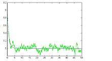
The graphic depicts a stochastic differential equation being solved using the Euler Scheme. The deterministic counterpart is shown as well.

Computer implementation

The following Python code implements Euler–Maruyama to solve the Ornstein–Uhlenbeck process

${\displaystyle dY_{t}=\theta \cdot (\mu -Y_{t})\,dt+\sigma \,dW_{t},\;\;Y_{0}=Y_{\mathrm {init} }.}$

The random numbers for $dW_{t}$ are generated using the numpy mathematics package.

import numpy as np
import matplotlib.pyplot as plt

num_sims = 5
N        = 1000

y_init = 0
t_init = 3
t_end  = 7

c_theta = 0.7
c_mu    = 1.5
c_sigma = 0.06

def mu(y, t): 
    return c_theta * (c_mu - y)
        
def sigma(y, t): 
    return c_sigma

dt   = float(t_end - t_init) / N
dW   = lambda dt: np.random.normal(loc = 0.0, scale = np.sqrt(dt))

t    = np.arange(t_init, t_end, dt)
y    = np.zeros(N)
y[0] = y_init

for i_sim in range(num_sims):
    for i in xrange(1, t.size):
        a = mu(y[i-1], (i-1) * dt)
        b = sigma(y[i-1], (i-1) * dt)
        y[i] = y[i-1] + a * dt + b * dW(dt)
    plt.plot(t, y)

plt.show()

See also

• Milstein method
• Runge–Kutta method (SDE)

Notes

1. Kloeden & Platen, 1992

References

• Kloeden, P.E. & Platen, E. (1992). Numerical Solution of Stochastic Differential Equations. Springer, Berlin. doi:10.1007/978-3-662-12616-5. ISBN 978-3-540-54062-5.