Wiener process

In mathematics, the Wiener process is a continuous-time stochastic process named in honor of Norbert Wiener. It is often called standard Brownian motion, after Robert Brown. It is one of the best known Lévy processes (càdlàg stochastic processes with stationary independent increments) and occurs frequently in pure and applied mathematics, economics, quantitative finance, and physics.
The Wiener process plays an important role both in pure and applied mathematics. In pure mathematics, the Wiener process gave rise to the study of continuous time martingales. It is a key process in terms of which more complicated stochastic processes can be described. As such, it plays a vital role in stochastic calculus, diffusion processes and even potential theory. It is the driving process of Schramm–Loewner evolution. In applied mathematics, the Wiener process is used to represent the integral of a white noise Gaussian process, and so is useful as a model of noise in electronics engineering (see Brownian noise), instrument errors in filtering theory and unknown forces in control theory.
The Wiener process has applications throughout the mathematical sciences. In physics it is used to study Brownian motion, the diffusion of minute particles suspended in fluid, and other types of diffusion via the Fokker–Planck and Langevin equations. It also forms the basis for the rigorous path integral formulation of quantum mechanics (by the Feynman–Kac formula, a solution to the Schrödinger equation can be represented in terms of the Wiener process) and the study of eternal inflation in physical cosmology. It is also prominent in the mathematical theory of finance, in particular the Black–Scholes option pricing model.
Characterisations of the Wiener process
The Wiener process Wt is characterised by the following properties:[1]
- W0 = 0 a.s.
- W has independent increments: Wt+u - Wt is independent of σ(Ws : s ≤ t) for u ≥ 0
- W has Gaussian increments: Wt+u - Wt is normally distributed with mean 0 and variance u, Wt+u−Wt ~ N(0, u)
- W has continuous paths: With probability 1, Wt is continuous in t.
The independent increments means that if 0 ≤ s1 < t1 ≤ s2 < t2 then Wt1−Ws1 and Wt2−Ws2 are independent random variables, and the similar condition holds for n increments.
An alternative characterisation of the Wiener process is the so-called Lévy characterisation that says that the Wiener process is an almost surely continuous martingale with W0 = 0 and quadratic variation [Wt, Wt] = t (which means that Wt2−t is also a martingale).
A third characterisation is that the Wiener process has a spectral representation as a sine series whose coefficients are independent N(0, 1) random variables. This representation can be obtained using the Karhunen–Loève theorem.
Another characterisation of a Wiener process is the Definite integral (from zero to time t) of a zero mean, unit variance, delta correlated ("white") Gaussian process.
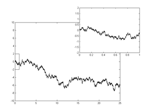
The Wiener process can be constructed as the scaling limit of a random walk, or other discrete-time stochastic processes with stationary independent increments. This is known as Donsker's theorem. Like the random walk, the Wiener process is recurrent in one or two dimensions (meaning that it returns almost surely to any fixed neighborhood of the origin infinitely often) whereas it is not recurrent in dimensions three and higher. Unlike the random walk, it is scale invariant, meaning that

is a Wiener process for any nonzero constant α. The Wiener measure is the probability law on the space of continuous functions g, with g(0) = 0, induced by the Wiener process. An integral based on Wiener measure may be called a Wiener integral.
Wiener process as a limit of random walk
Let be i.i.d. random variables with mean 0 and variance 1. For each n, define a continuous time stochastic process


This is a random step function. Increments of are independent because the are independent. For large n, is close to by the central limit theorem. It's tempting to believe that as , will approach a Wiener process, and this temptation bears true fruit. The proof is provided by Donsker's theorem. This formulation explained why Brownian motion is ubiquitous.[2]


Properties of a one-dimensional Wiener process
Basic properties
The unconditional probability density function, which follows normal distribution with mean = 0 and variance = t, at a fixed time t:

The expectation is zero:
![E[W_{t}]=0.](../I/m/8b1ba46ce18f203f1dfd7a1e2701f4cb938dfb5d.svg)
The variance, using the computational formula, is t:
![\operatorname {Var} (W_{t})=E\left[W_{t}^{2}\right]-E^{2}[W_{t}]=E\left[W_{t}^{2}\right]-0=E\left[W_{t}^{2}\right]=t.](../I/m/cb3510130f603bd2f48b5530c06f4cde8ca25250.svg)
Covariance and correlation
The covariance and correlation:


The results for the expectation and variance follow immediately from the definition that increments have a normal distribution, centered at zero. Thus

The results for the covariance and correlation follow from the definition that non-overlapping increments are independent, of which only the property that they are uncorrelated is used. Suppose that t1 < t2.
![{\displaystyle \operatorname {cov} (W_{t_{1}},W_{t_{2}})=\operatorname {E} \left[(W_{t_{1}}-\operatorname {E} [W_{t_{1}}])\cdot (W_{t_{2}}-\operatorname {E} [W_{t_{2}}])\right]=\operatorname {E} \left[W_{t_{1}}\cdot W_{t_{2}}\right].}](../I/m/fbb2a5668da12af0e735a0c8dce59ec570bbb30d.svg)
Substituting

we arrive at:
![{\displaystyle {\begin{aligned}\operatorname {E} [W_{t_{1}}\cdot W_{t_{2}}]&=\operatorname {E} \left[W_{t_{1}}\cdot ((W_{t_{2}}-W_{t_{1}})+W_{t_{1}})\right]\\&=\operatorname {E} \left[W_{t_{1}}\cdot (W_{t_{2}}-W_{t_{1}})\right]+\operatorname {E} \left[W_{t_{1}}^{2}\right].\end{aligned}}}](../I/m/2fbe8fb9bb18a4ec1a9af1844c268d825436ad22.svg)
Since W(t1) = W(t1) − W(t0) and W(t2) − W(t1), are independent,
![{\displaystyle \operatorname {E} \left[W_{t_{1}}\cdot (W_{t_{2}}-W_{t_{1}})\right]=\operatorname {E} [W_{t_{1}}]\cdot \operatorname {E} [W_{t_{2}}-W_{t_{1}}]=0.}](../I/m/8c77aa89414719e3c1db8c93475c1521da8be480.svg)
Thus
![{\displaystyle \operatorname {cov} (W_{t_{1}},W_{t_{2}})=\operatorname {E} \left[W_{t_{1}}^{2}\right]=t_{1}.}](../I/m/0b56dd00bf0345dd58627cabd374ca58aabc40b8.svg)
Wiener representation
Wiener (1923) also gave a representation of a Brownian path in terms of a random Fourier series. If are independent Gaussian variables with mean zero and variance one, then


and

represent a Brownian motion on . The scaled process
![[0,1]](../I/m/738f7d23bb2d9642bab520020873cccbef49768d.svg)

is a Brownian motion on (cf. Karhunen–Loève theorem).
![[0,c]](../I/m/d8f04abeab39818aa786f2e5f9cdf163379e60c6.svg)
Running maximum
The joint distribution of the running maximum

and Wt is

To get the unconditional distribution of , integrate over −∞ < w ≤ m :

![{\displaystyle {\begin{aligned}f_{M_{t}}(m)&=\int _{-\infty }^{m}f_{M_{t},W_{t}}(m,w)\,dw=\int _{-\infty }^{m}{\frac {2(2m-w)}{t{\sqrt {2\pi t}}}}e^{-{\frac {(2m-w)^{2}}{2t}}}\,dw\\[5pt]&={\sqrt {\frac {2}{\pi t}}}e^{-{\frac {m^{2}}{2t}}},\qquad m\geq 0.\end{aligned}}}](../I/m/e7f7b6fcc95237f01f282fbcb0140af95f4f2598.svg)
And the expectation[3]
![{\displaystyle \operatorname {E} [M_{t}]=\int _{0}^{\infty }mf_{M_{t}}(m)\,dm=\int _{0}^{\infty }m{\sqrt {\frac {2}{\pi t}}}e^{-{\frac {m^{2}}{2t}}}\,dm={\sqrt {\frac {2t}{\pi }}}}](../I/m/b6bc0f61007dd872ee5fce91d4189001979a8528.svg)
Self-similarity

Brownian scaling
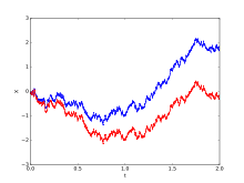
For every c > 0 the process is another Wiener process.
Time reversal
The process for 0 ≤ t ≤ 1 is distributed like Wt for 0 ≤ t ≤ 1.

Time inversion
The process is another Wiener process.

A class of Brownian martingales
If a polynomial p(x, t) satisfies the PDE

then the stochastic process

is a martingale.
Example: is a martingale, which shows that the quadratic variation of W on [0, t] is equal to t. It follows that the expected time of first exit of W from (−c, c) is equal to c2.

More generally, for every polynomial p(x, t) the following stochastic process is a martingale:

where a is the polynomial

Example: the process


is a martingale, which shows that the quadratic variation of the martingale on [0, t] is equal to

About functions p(xa, t) more general than polynomials, see local martingales.
Some properties of sample paths
The set of all functions w with these properties is of full Wiener measure. That is, a path (sample function) of the Wiener process has all these properties almost surely.
Qualitative properties
- For every ε > 0, the function w takes both (strictly) positive and (strictly) negative values on (0, ε).
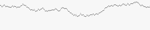
- The function w is continuous everywhere but differentiable nowhere (like the Weierstrass function).
- Points of local maximum of the function w are a dense countable set; the maximum values are pairwise different; each local maximum is sharp in the following sense: if w has a local maximum at t then
- The same holds for local minima.

- The function w has no points of local increase, that is, no t > 0 satisfies the following for some ε in (0, t): first, w(s) ≤ w(t) for all s in (t − ε, t), and second, w(s) ≥ w(t) for all s in (t, t + ε). (Local increase is a weaker condition than that w is increasing on (t − ε, t + ε).) The same holds for local decrease.
- The function w is of unbounded variation on every interval.
- The quadratic variation of w over [0,t] is t.
- Zeros of the function w are a nowhere dense perfect set of Lebesgue measure 0 and Hausdorff dimension 1/2 (therefore, uncountable).
Quantitative properties
Law of the iterated logarithm

Modulus of continuity
Local modulus of continuity:

Global modulus of continuity (Lévy):

Local time
The image of the Lebesgue measure on [0, t] under the map w (the pushforward measure) has a density Lt(·). Thus,

for a wide class of functions f (namely: all continuous functions; all locally integrable functions; all non-negative measurable functions). The density Lt is (more exactly, can and will be chosen to be) continuous. The number Lt(x) is called the local time at x of w on [0, t]. It is strictly positive for all x of the interval (a, b) where a and b are the least and the greatest value of w on [0, t], respectively. (For x outside this interval the local time evidently vanishes.) Treated as a function of two variables x and t, the local time is still continuous. Treated as a function of t (while x is fixed), the local time is a singular function corresponding to a nonatomic measure on the set of zeros of w.
These continuity properties are fairly non-trivial. Consider that the local time can also be defined (as the density of the pushforward measure) for a smooth function. Then, however, the density is discontinuous, unless the given function is monotone. In other words, there is a conflict between good behavior of a function and good behavior of its local time. In this sense, the continuity of the local time of the Wiener process is another manifestation of non-smoothness of the trajectory.
Related processes
The stochastic process defined by

is called a Wiener process with drift μ and infinitesimal variance σ2. These processes exhaust continuous Lévy processes.
Two random processes on the time interval [0, 1] appear, roughly speaking, when conditioning the Wiener process to vanish on both ends of [0,1]. With no further conditioning, the process takes both positive and negative values on [0, 1] and is called Brownian bridge. Conditioned also to stay positive on (0, 1), the process is called Brownian excursion.[4] In both cases a rigorous treatment involves a limiting procedure, since the formula P(A|B) = P(A ∩ B)/P(B) does not apply when P(B) = 0.
A geometric Brownian motion can be written

It is a stochastic process which is used to model processes that can never take on negative values, such as the value of stocks.
The stochastic process

is distributed like the Ornstein–Uhlenbeck process.
The time of hitting a single point x > 0 by the Wiener process is a random variable with the Lévy distribution. The family of these random variables (indexed by all positive numbers x) is a left-continuous modification of a Lévy process. The right-continuous modification of this process is given by times of first exit from closed intervals [0, x].
The local time L = (Lxt)x ∈ R, t ≥ 0 of a Brownian motion describes the time that the process spends at the point x. Formally

where δ is the Dirac delta function. The behaviour of the local time is characterised by Ray–Knight theorems.
Brownian martingales
Let A be an event related to the Wiener process (more formally: a set, measurable with respect to the Wiener measure, in the space of functions), and Xt the conditional probability of A given the Wiener process on the time interval [0, t] (more formally: the Wiener measure of the set of trajectories whose concatenation with the given partial trajectory on [0, t] belongs to A). Then the process Xt is a continuous martingale. Its martingale property follows immediately from the definitions, but its continuity is a very special fact – a special case of a general theorem stating that all Brownian martingales are continuous. A Brownian martingale is, by definition, a martingale adapted to the Brownian filtration; and the Brownian filtration is, by definition, the filtration generated by the Wiener process.
Integrated Brownian motion
The time-integral of the Wiener process

is called integrated Brownian motion or integrated Wiener process. It arises in many applications and can be shown to have the distribution N(0, t3/3), calculus lead using the fact that the covariance of the Wiener process is .[5]

Time change
Every continuous martingale (starting at the origin) is a time changed Wiener process.
Example: 2Wt = V(4t) where V is another Wiener process (different from W but distributed like W).
Example. where and V is another Wiener process.


In general, if M is a continuous martingale then where A(t) is the quadratic variation of M on [0, t], and V is a Wiener process.

Corollary. (See also Doob's martingale convergence theorems) Let Mt be a continuous martingale, and


Then only the following two cases are possible:


other cases (such as etc.) are of probability 0.


Especially, a nonnegative continuous martingale has a finite limit (as t → ∞) almost surely.
All stated (in this subsection) for martingales holds also for local martingales.
Change of measure
A wide class of continuous semimartingales (especially, of diffusion processes) is related to the Wiener process via a combination of time change and change of measure.
Using this fact, the qualitative properties stated above for the Wiener process can be generalized to a wide class of continuous semimartingales.[6][7]
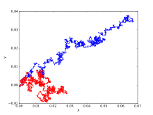
Complex-valued Wiener process
The complex-valued Wiener process may be defined as a complex-valued random process of the form Zt = Xt + iYt where Xt, Yt are independent Wiener processes (real-valued).[8]
Self-similarity
Brownian scaling, time reversal, time inversion: the same as in the real-valued case.
Rotation invariance: for every complex number c such that |c| = 1 the process cZt is another complex-valued Wiener process.
Time change
If f is an entire function then the process is a time-changed complex-valued Wiener process.

Example: where


and U is another complex-valued Wiener process.
In contrast to the real-valued case, a complex-valued martingale is generally not a time-changed complex-valued Wiener process. For example, the martingale 2Xt + iYt is not (here Xt, Yt are independent Wiener processes, as before).
See also
Numerical path sampling: |
Notes
- ↑ Durrett 1996, Sect. 7.1
- ↑ Steven Lalley, Mathematical Finance 345 Lecture 5: Brownian Motion (2001)
- ↑ Shreve, Steven E (2008). Stochastic Calculus for Finance II: Continuous Time Models. Springer. p. 114. ISBN 978-0-387-40101-0.
- ↑ Vervaat, W. (1979). "A relation between Brownian bridge and Brownian excursion". Annals of Probability. 7 (1): 143–149. doi:10.1214/aop/1176995155. JSTOR 2242845.
- ↑ Forum, "Variance of integrated Wiener process", 2009.
- ↑ Revuz, D., & Yor, M. (1999). Continuous martingales and Brownian motion (Vol. 293). Springer.
- ↑ Doob, J. L. (1953). Stochastic processes (Vol. 101). Wiley: New York.
- ↑ Navarro-moreno, J.; Estudillo-martinez, M.D; Fernandez-alcala, R.M.; Ruiz-molina, J.C. (2009), "Estimation of Improper Complex-Valued Random Signals in Colored Noise by Using the Hilbert Space Theory" (PDF), IEEE Transactions on Information Theory, 55 (6): 2859–2867, doi:10.1109/TIT.2009.2018329, retrieved 2010-03-30
References
- Kleinert, Hagen (2004). Path Integrals in Quantum Mechanics, Statistics, Polymer Physics, and Financial Markets (4th ed.). Singapore: World Scientific. ISBN 981-238-107-4. (also available online: PDF-files)
- Stark, Henry; Woods, John (2002). Probability and Random Processes with Applications to Signal Processing (3rd ed.). New Jersey: Prentice Hall. ISBN 0-13-020071-9.
- Durrett, R. (2000). Probability: theory and examples (4th ed.). Cambridge University Press. ISBN 0-521-76539-0.
- Revuz, Daniel; Yor, Marc (1994). Continuous martingales and Brownian motion (Second ed.). Springer-Verlag.
External links
- Brownian motion java simulation
- Article for the school-going child
- Brownian Motion, "Diverse and Undulating"
- Discusses history, botany and physics of Brown's original observations, with videos
- "Einstein's prediction finally witnessed one century later" : a test to observe the velocity of Brownian motion
- "Interactive Web Application: Stochastic Processes used in Quantitative Finance".