Hilbert curve

View first 10 iterations
A Hilbert curve (also known as a Hilbert space-filling curve) is a continuous fractal space-filling curve first described by the German mathematician David Hilbert in 1891,[1] as a variant of the space-filling Peano curves discovered by Giuseppe Peano in 1890.[2]
Because it is space-filling, its Hausdorff dimension is (precisely, its image is the unit square, whose dimension is 2 in any definition of dimension; its graph is a compact set homeomorphic to the closed unit interval, with Hausdorff dimension 2).

is the th approximation to the limiting curve. The Euclidean length of is , i.e., it grows exponentially with , while at the same time always being bounded by a square with a finite area.


Images
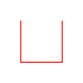 Hilbert curve, first order
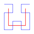 Hilbert curves, first and second orders
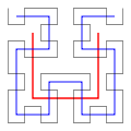 Hilbert curves, first to third orders
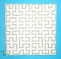 String art
 Hilbert curve, construction color-coded
 A Hilbert curve in three dimensions
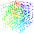 A 3-D Hilbert curve with color showing progression
 This GIF file displays an animation of circles traveling along the path of a Hilbert Space filling Curve.
Applications and mapping algorithms
Both the true Hilbert curve and its discrete approximations are useful because they give a mapping between 1D and 2D space that fairly well preserves locality.[3] If (x,y) are the coordinates of a point within the unit square, and d is the distance along the curve when it reaches that point, then points that have nearby d values will also have nearby (x,y) values. The converse can't always be true. There will sometimes be points where the (x,y) coordinates are close but their d values are far apart.
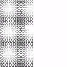
Because of this locality property, the Hilbert curve is widely used in computer science. For example, the range of IP addresses used by computers can be mapped into a picture using the Hilbert curve. Code to generate the image would map from 2D to 1D to find the color of each pixel, and the Hilbert curve is sometimes used because it keeps nearby IP addresses close to each other in the picture.
A grayscale photograph can be converted to a dithered black-and-white image using thresholding, with the leftover amount from each pixel added to the next pixel along the Hilbert curve. Code to do this would map from 1D to 2D, and the Hilbert curve is sometimes used because it does not create the distracting patterns that would be visible to the eye if the order were simply left to right across each row of pixels. Hilbert curves in higher dimensions are an instance of a generalization of Gray codes, and are sometimes used for similar purposes, for similar reasons. For multidimensional databases, Hilbert order has been proposed to be used instead of Z order because it has better locality-preserving behavior. For example, Hilbert curves have been used to compress and accelerate R-tree indexes[4] (see Hilbert R-tree). They have also been used to help compress data warehouses.[5][6]
Given the variety of applications, it is useful to have algorithms to map in both directions. In many languages, these are better if implemented with iteration rather than recursion. The following C code performs the mappings in both directions, using iteration and bit operations rather than recursion. It assumes a square divided into n by n cells, for n a power of 2, with integer coordinates, with (0,0) in the lower left corner, (n-1,n-1) in the upper right corner, and a distance d that starts at 0 in the lower left corner and goes to in the lower-right corner.

//convert (x,y) to d
int xy2d (int n, int x, int y) {
    int rx, ry, s, d=0;
    for (s=n/2; s>0; s/=2) {
        rx = (x & s) > 0;
        ry = (y & s) > 0;
        d += s * s * ((3 * rx) ^ ry);
        rot(s, &x, &y, rx, ry);
    }
    return d;
}

//convert d to (x,y)
void d2xy(int n, int d, int *x, int *y) {
    int rx, ry, s, t=d;
    *x = *y = 0;
    for (s=1; s<n; s*=2) {
        rx = 1 & (t/2);
        ry = 1 & (t ^ rx);
        rot(s, x, y, rx, ry);
        *x += s * rx;
        *y += s * ry;
        t /= 4;
    }
}

//rotate/flip a quadrant appropriately
void rot(int n, int *x, int *y, int rx, int ry) {
    if (ry == 0) {
        if (rx == 1) {
            *x = n-1 - *x;
            *y = n-1 - *y;
        }

        //Swap x and y
        int t  = *x;
        *x = *y;
        *y = t;
    }
}
These use the C conventions: the & symbol is a bitwise AND, the ^ symbol is a bitwise XOR, the += operator adds on to a variable, and the /= operator divides a variable. The handling of booleans in C means that in xy2d, the variable rx is set to 0 or 1 to match bit s of x, and similarly for ry.
The xy2d function works top down, starting with the most significant bits of x and y, and building up the most significant bits of d first. The d2xy function works in the opposite order, starting with the least significant bits of d, and building up x and y starting with the least significant bits. Both functions use the rotation function to rotate and flip the (x,y) coordinate system appropriately.
The two mapping algorithms work in similar ways. The entire square is viewed as composed of 4 regions, arranged 2 by 2. Each region is composed of 4 smaller regions, and so on, for a number of levels. At level s, each region is s by s cells. There is a single FOR loop that iterates through levels. On each iteration, an amount is added to d or to x and y, determined by which of the 4 regions it is in at the current level. The current region out of the 4 is (rx,ry), where rx and ry are each 0 or 1. So it consumes 2 input bits, (either 2 from d or 1 each from x and y), and generates two output bits. It also calls the rotation function so that (x,y) will be appropriate for the next level, on the next iteration. For xy2d, it starts at the top level of the entire square, and works its way down to the lowest level of individual cells. For d2xy, it starts at the bottom with cells, and works up to include the entire square.
It is possible to implement Hilbert curves efficiently even when the data space does not form a square.[7] Moreover, there are several possible generalizations of Hilbert curves to higher dimensions.[8][9]
Representation as Lindenmayer system
The Hilbert Curve can be expressed by a rewrite system (L-system).
- Alphabet : A, B
- Constants : F + −
- Axiom : A
- Production rules:
- A → − B F + A F A + F B −
- B → + A F − B F B − F A +
Here, "F" means "draw forward", "−" means "turn left 90°", "+" means "turn right 90°" (see turtle graphics), and "A" and "B" are ignored during drawing.
Other implementations
Arthur Butz[10] provided an algorithm for calculating the Hilbert curve in multidimensions.
Graphics Gems II[11] discusses Hilbert Curve coherency, and provides implementation.
See also
| Wikimedia Commons has media related to Hilbert curve. |
- Hilbert curve scheduling
- Hilbert R-tree
- Sierpiński curve
- Moore curve
- Space-filling curves
- List of fractals by Hausdorff dimension
Notes
- ↑ D. Hilbert: Über die stetige Abbildung einer Linie auf ein Flächenstück. Mathematische Annalen 38 (1891), 459–460.
- ↑ G.Peano: Sur une courbe, qui remplit toute une aire plane. Mathematische Annalen 36 (1890), 157–160.
- ↑ Moon, B.; Jagadish, H.V.; Faloutsos, C.; Saltz, J.H. (2001), "Analysis of the clustering properties of the Hilbert space-filling curve", IEEE Transactions on Knowledge and Data Engineering, 13 (1): 124–141, doi:10.1109/69.908985.
- ↑ I. Kamel, C. Faloutsos, Hilbert R-tree: An improved R-tree using fractals, in: Proceedings of the 20th International Conference on Very Large Data Bases, Morgan Kaufmann Publishers Inc., San Francisco, CA, USA, 1994, pp. 500–509.
- ↑ Eavis, T.; Cueva, D. (2007). "A Hilbert space compression architecture for data warehouse environments". Lecture Notes in Computer Science. 4654: 1–12.
- ↑ Lemire, Daniel; Kaser, Owen (2011). "Reordering Columns for Smaller Indexes". Information Sciences. 181 (12). arXiv:0909.1346
 .
. - ↑ Hamilton, C. H.; Rau-Chaplin, A. (2007). "Compact Hilbert indices: Space-filling curves for domains with unequal side lengths". Information Processing Letters. 105 (5): 155–163. doi:10.1016/j.ipl.2007.08.034.
- ↑ Alber, J.; Niedermeier, R. (2000). "On multidimensional curves with Hilbert property". Theory of Computing Systems. 33 (4): 295–312. doi:10.1007/s002240010003.
- ↑ H. J. Haverkort, F. van Walderveen, Four-dimensional Hilbert curves for R-trees, in: Proceedings of the Eleventh Workshop on Algorithm Engineering and Experiments, 2009, pp. 63–73.
- ↑ A.R. Butz (April 1971). "Alternative algorithm for Hilbert's space filling curve.". IEEE Transactions on Computers. 20: 424–42. doi:10.1109/T-C.1971.223258.
- ↑ Voorhies, Douglas: Space-Filling Curves and a Measure of Coherence, p. 26-30, Graphics Gems II.
External links
- Dynamic Hilbert curve with JSXGraph
- Three.js WebGL 3D Hilbert curve demo
- XKCD cartoon using the locality properties of the Hilbert curve to create a "map of the internet"
- Gcode generator for Hilbert curve
- Iterative algorithm for drawing Hilbert curve in JavaScript