Johnson's algorithm
| Class | All-pairs shortest path problem (for weighted graphs) |
|---|---|
| Data structure | Graph |
| Worst-case performance |

| Graph and tree search algorithms |
|---|
| Listings |
|
| Related topics |
Johnson's algorithm is a way to find the shortest paths between all pairs of vertices in a sparse, edge weighted, directed graph. It allows some of the edge weights to be negative numbers, but no negative-weight cycles may exist. It works by using the Bellman–Ford algorithm to compute a transformation of the input graph that removes all negative weights, allowing Dijkstra's algorithm to be used on the transformed graph.[1][2] It is named after Donald B. Johnson, who first published the technique in 1977.[3]
A similar reweighting technique is also used in Suurballe's algorithm for finding two disjoint paths of minimum total length between the same two vertices in a graph with non-negative edge weights.[4]
Algorithm description
Johnson's algorithm consists of the following steps:[1][2]
- First, a new node q is added to the graph, connected by zero-weight edges to each of the other nodes.
- Second, the Bellman–Ford algorithm is used, starting from the new vertex q, to find for each vertex v the minimum weight h(v) of a path from q to v. If this step detects a negative cycle, the algorithm is terminated.
- Next the edges of the original graph are reweighted using the values computed by the Bellman–Ford algorithm: an edge from u to v, having length w(u,v), is given the new length w(u,v) + h(u) − h(v).
- Finally, q is removed, and Dijkstra's algorithm is used to find the shortest paths from each node s to every other vertex in the reweighted graph.
Example
The first three stages of Johnson's algorithm are depicted in the illustration below.
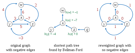
The graph on the left of the illustration has two negative edges, but no negative cycles. At the center is shown the new vertex q, a shortest path tree as computed by the Bellman–Ford algorithm with q as starting vertex, and the values h(v) computed at each other node as the length of the shortest path from q to that node. Note that these values are all non-positive, because q has a length-zero edge to each vertex and the shortest path can be no longer than that edge. On the right is shown the reweighted graph, formed by replacing each edge weight w(u,v) by w(u,v) + h(u) − h(v). In this reweighted graph, all edge weights are non-negative, but the shortest path between any two nodes uses the same sequence of edges as the shortest path between the same two nodes in the original graph. The algorithm concludes by applying Dijkstra's algorithm to each of the four starting nodes in the reweighted graph.
Correctness
In the reweighted graph, all paths between a pair s and t of nodes have the same quantity h(s) − h(t) added to them. The previous statement can be proven as follows: Let p be an s-t path. Its weight W in the reweighted graph is given by the following expression:

Every is cancelled by in the previous bracketed expression; therefore, we are left with the following expression for W:


The bracketed expression is the weight of p in the original weighting.
Since the reweighting adds the same amount to the weight of every s-t path, a path is a shortest path in the original weighting if and only if it is a shortest path after reweighting. The weight of edges that belong to a shortest path from q to any node is zero, and therefore the lengths of the shortest paths from q to every node become zero in the reweighted graph; however, they still remain shortest paths. Therefore, there can be no negative edges: if edge uv had a negative weight after the reweighting, then the zero-length path from q to u together with this edge would form a negative-length path from q to v, contradicting the fact that all vertices have zero distance from q. The non-existence of negative edges ensures the optimality of the paths found by Dijkstra's algorithm. The distances in the original graph may be calculated from the distances calculated by Dijkstra's algorithm in the reweighted graph by reversing the reweighting transformation.[1]
Analysis
The time complexity of this algorithm, using Fibonacci heaps in the implementation of Dijkstra's algorithm, is : the algorithm uses time for the Bellman–Ford stage of the algorithm, and for each of the instantiations of Dijkstra's algorithm. Thus, when the graph is sparse, the total time can be faster than the Floyd–Warshall algorithm, which solves the same problem in time .[1]


References
- 1 2 3 4 Cormen, Thomas H.; Leiserson, Charles E.; Rivest, Ronald L.; Stein, Clifford (2001), Introduction to Algorithms, MIT Press and McGraw-Hill, ISBN 978-0-262-03293-3. Section 25.3, "Johnson's algorithm for sparse graphs", pp. 636–640.
- 1 2 Black, Paul E. (2004), "Johnson's Algorithm", Dictionary of Algorithms and Data Structures, National Institute of Standards and Technology.
- ↑ Johnson, Donald B. (1977), "Efficient algorithms for shortest paths in sparse networks", Journal of the ACM, 24 (1): 1–13, doi:10.1145/321992.321993.
- ↑ Suurballe, J. W. (1974), "Disjoint paths in a network", Networks, 14 (2): 125–145, doi:10.1002/net.3230040204.