Mathematical formulation of quantum mechanics

The mathematical formulations of quantum mechanics are those mathematical formalisms that permit a rigorous description of quantum mechanics. Such are distinguished from mathematical formalisms for theories developed prior to the early 1900s by the use of abstract mathematical structures, such as infinite-dimensional Hilbert spaces and operators on these spaces. Many of these structures are drawn from functional analysis, a research area within pure mathematics that was influenced in part by the needs of quantum mechanics. In brief, values of physical observables such as energy and momentum were no longer considered as values of functions on phase space, but as eigenvalues; more precisely as spectral values of linear operators in Hilbert space.[1]
These formulations of quantum mechanics continue to be used today. At the heart of the description are ideas of quantum state and quantum observable which are radically different from those used in previous models of physical reality. While the mathematics permits calculation of many quantities that can be measured experimentally, there is a definite theoretical limit to values that can be simultaneously measured. This limitation was first elucidated by Heisenberg through a thought experiment, and is represented mathematically in the new formalism by the non-commutativity of operators representing quantum observables.
Prior to the emergence of quantum mechanics as a separate theory, the mathematics used in physics consisted mainly of formal mathematical analysis, beginning with calculus, and increasing in complexity up to differential geometry and partial differential equations. Probability theory was used in statistical mechanics. Geometric intuition played a strong role in the first two and, accordingly, theories of relativity were formulated entirely in terms of geometric concepts. The phenomenology of quantum physics arose roughly between 1895 and 1915, and for the 10 to 15 years before the emergence of quantum theory (around 1925) physicists continued to think of quantum theory within the confines of what is now called classical physics, and in particular within the same mathematical structures. The most sophisticated example of this is the Sommerfeld–Wilson–Ishiwara quantization rule, which was formulated entirely on the classical phase space.
History of the formalism
The "old quantum theory" and the need for new mathematics
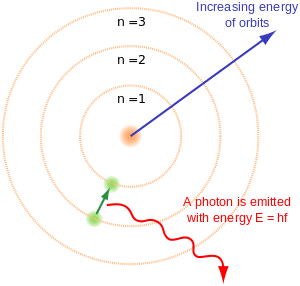
In the 1890s, Planck was able to derive the blackbody spectrum which was later used to avoid the classical ultraviolet catastrophe by making the unorthodox assumption that, in the interaction of electromagnetic radiation with matter, energy could only be exchanged in discrete units which he called quanta. Planck postulated a direct proportionality between the frequency of radiation and the quantum of energy at that frequency. The proportionality constant, h, is now called Planck's constant in his honor.
In 1905, Einstein explained certain features of the photoelectric effect by assuming that Planck's energy quanta were actual particles, which were later dubbed photons.
All of these developments were phenomenological and challenged the theoretical physics of the time. Bohr and Sommerfeld went on to modify classical mechanics in an attempt to deduce the Bohr model from first principles. They proposed that, of all closed classical orbits traced by a mechanical system in its phase space, only the ones that enclosed an area which was a multiple of Planck's constant were actually allowed. The most sophisticated version of this formalism was the so-called Sommerfeld–Wilson–Ishiwara quantization. Although the Bohr model of the hydrogen atom could be explained in this way, the spectrum of the helium atom (classically an unsolvable 3-body problem) could not be predicted. The mathematical status of quantum theory remained uncertain for some time.
In 1923 de Broglie proposed that wave–particle duality applied not only to photons but to electrons and every other physical system.
The situation changed rapidly in the years 1925–1930, when working mathematical foundations were found through the groundbreaking work of Erwin Schrödinger, Werner Heisenberg, Max Born, Pascual Jordan, and the foundational work of John von Neumann, Hermann Weyl and Paul Dirac, and it became possible to unify several different approaches in terms of a fresh set of ideas. The physical interpretation of the theory was also clarified in these years after Werner Heisenberg discovered the uncertainty relations and Niels Bohr introduced the idea of complementarity.
The "new quantum theory"
Werner Heisenberg's matrix mechanics was the first successful attempt at replicating the observed quantization of atomic spectra. Later in the same year, Schrödinger created his wave mechanics. Schrödinger's formalism was considered easier to understand, visualize and calculate as it led to differential equations, which physicists were already familiar with solving. Within a year, it was shown that the two theories were equivalent.
Schrödinger himself initially did not understand the fundamental probabilistic nature of quantum mechanics, as he thought that the absolute square of the wave function of an electron should be interpreted as the charge density of an object smeared out over an extended, possibly infinite, volume of space. It was Max Born who introduced the interpretation of the absolute square of the wave function as the probability distribution of the position of a pointlike object. Born's idea was soon taken over by Niels Bohr in Copenhagen who then became the "father" of the Copenhagen interpretation of quantum mechanics. Schrödinger's wave function can be seen to be closely related to the classical Hamilton–Jacobi equation. The correspondence to classical mechanics was even more explicit, although somewhat more formal, in Heisenberg's matrix mechanics. In his PhD thesis project, Paul Dirac[2] discovered that the equation for the operators in the Heisenberg representation, as it is now called, closely translates to classical equations for the dynamics of certain quantities in the Hamiltonian formalism of classical mechanics, when one expresses them through Poisson brackets, a procedure now known as canonical quantization.
To be more precise, already before Schrödinger, the young postdoctoral fellow Werner Heisenberg invented his matrix mechanics, which was the first correct quantum mechanics–– the essential breakthrough. Heisenberg's matrix mechanics formulation was based on algebras of infinite matrices, a very radical formulation in light of the mathematics of classical physics, although he started from the index-terminology of the experimentalists of that time, not even aware that his "index-schemes" were matrices, as Born soon pointed out to him. In fact, in these early years, linear algebra was not generally popular with physicists in its present form.
Although Schrödinger himself after a year proved the equivalence of his wave-mechanics and Heisenberg's matrix mechanics, the reconciliation of the two approaches and their modern abstraction as motions in Hilbert space is generally attributed to Paul Dirac, who wrote a lucid account in his 1930 classic The Principles of Quantum Mechanics. He is the third, and possibly most important, pillar of that field (he soon was the only one to have discovered a relativistic generalization of the theory). In his above-mentioned account, he introduced the bra–ket notation, together with an abstract formulation in terms of the Hilbert space used in functional analysis; he showed that Schrödinger's and Heisenberg's approaches were two different representations of the same theory, and found a third, most general one, which represented the dynamics of the system. His work was particularly fruitful in all kinds of generalizations of the field.
The first complete mathematical formulation of this approach, known as the Dirac–von Neumann axioms, is generally credited to John von Neumann's 1932 book Mathematical Foundations of Quantum Mechanics, although Hermann Weyl had already referred to Hilbert spaces (which he called unitary spaces) in his 1927 classic paper and book. It was developed in parallel with a new approach to the mathematical spectral theory based on linear operators rather than the quadratic forms that were David Hilbert's approach a generation earlier. Though theories of quantum mechanics continue to evolve to this day, there is a basic framework for the mathematical formulation of quantum mechanics which underlies most approaches and can be traced back to the mathematical work of John von Neumann. In other words, discussions about interpretation of the theory, and extensions to it, are now mostly conducted on the basis of shared assumptions about the mathematical foundations.
Later developments
The application of the new quantum theory to electromagnetism resulted in quantum field theory, which was developed starting around 1930. Quantum field theory has driven the development of more sophisticated formulations of quantum mechanics, of which the one presented here is a simple special case.
- Path integral formulation
- Phase space formulation of Quantum Mechanics & geometric quantization
- Signed Particle Formulation[3]
- quantum field theory in curved spacetime
- axiomatic, algebraic and constructive quantum field theory
- C* algebra formalism
- Generalized Statistical Model of Quantum Mechanics
On a different front, von Neumann originally dispatched quantum measurement with his infamous postulate on the collapse of the wavefunction, raising a host of philosophical problems. Over the intervening 70 years, the problem of measurement became an active research area and itself spawned some new formulations of quantum mechanics.
- Relative state/Many-worlds interpretation of quantum mechanics
- Decoherence
- Consistent histories formulation of quantum mechanics
- Quantum logic formulation of quantum mechanics
A related topic is the relationship to classical mechanics. Any new physical theory is supposed to reduce to successful old theories in some approximation. For quantum mechanics, this translates into the need to study the so-called classical limit of quantum mechanics. Also, as Bohr emphasized, human cognitive abilities and language are inextricably linked to the classical realm, and so classical descriptions are intuitively more accessible than quantum ones. In particular, quantization, namely the construction of a quantum theory whose classical limit is a given and known classical theory, becomes an important area of quantum physics in itself.
Finally, some of the originators of quantum theory (notably Einstein and Schrödinger) were unhappy with what they thought were the philosophical implications of quantum mechanics. In particular, Einstein took the position that quantum mechanics must be incomplete, which motivated research into so-called hidden-variable theories. The issue of hidden variables has become in part an experimental issue with the help of quantum optics.
- de Broglie–Bohm–Bell pilot wave formulation of quantum mechanics
- Bell's inequalities
- Kochen–Specker theorem
Mathematical structure of quantum mechanics
A physical system is generally described by three basic ingredients: states; observables; and dynamics (or law of time evolution) or, more generally, a group of physical symmetries. A classical description can be given in a fairly direct way by a phase space model of mechanics: states are points in a symplectic phase space, observables are real-valued functions on it, time evolution is given by a one-parameter group of symplectic transformations of the phase space, and physical symmetries are realized by symplectic transformations. A quantum description consists of a Hilbert space of states, observables are self adjoint operators on the space of states, time evolution is given by a one-parameter group of unitary transformations on the Hilbert space of states, and physical symmetries are realized by unitary transformations.
Postulates of quantum mechanics
The following summary of the mathematical framework of quantum mechanics can be partly traced back to the Dirac–von Neumann axioms.
- Each physical system is associated with a (topologically) separable complex Hilbert space H with inner product . Rays (one-dimensional subspaces) in H are associated with states of the system. In other words, physical states can be identified with equivalence classes of vectors of length 1 in H, where two vectors represent the same state if they differ only by a phase factor. Separability is a mathematically convenient hypothesis, with the physical interpretation that countably many observations are enough to uniquely determine the state. A quantum mechanical state is a ray in projective Hilbert space, not a vector. Many textbooks fail to make this distinction, which could be partly a result of the fact that the Schrödinger equation itself involves Hilbert-space "vectors", with the result that the imprecise use of "state vector" rather than ray is very difficult to avoid.[4]
- The Hilbert space of a composite system is the Hilbert space tensor product of the state spaces associated with the component systems (for instance, J.M. Jauch, Foundations of quantum mechanics, section 11-7). For a non-relativistic system consisting of a finite number of distinguishable particles, the component systems are the individual particles.
- Physical symmetries act on the Hilbert space of quantum states unitarily or antiunitarily due to Wigner's theorem (supersymmetry is another matter entirely).
- Physical observables are represented by Hermitian matrices on H.
- The expectation value (in the sense of probability theory) of the observable A for the system in state represented by the unit vector ψ ∈ H is
- By spectral theory, we can associate a probability measure to the values of A in any state ψ. We can also show that the possible values of the observable A in any state must belong to the spectrum of A. In the special case A has only discrete spectrum, the possible outcomes of measuring A are its eigenvalues. More precisely, if we represent the state ψ in the basis formed by the eigenvectors of A, then the square of the modulus of the component attached to a given eigenvector is the probability of observing its corresponding eigenvalue.

- More generally, a state can be represented by a so-called density operator, which is a trace class, nonnegative self-adjoint operator ρ normalized to be of trace 1. The expected value of A in the state ρ is
- If ρψ is the orthogonal projector onto the one-dimensional subspace of H spanned by |ψ⟩, then
- Density operators are those that are in the closure of the convex hull of the one-dimensional orthogonal projectors. Conversely, one-dimensional orthogonal projectors are extreme points of the set of density operators. Physicists also call one-dimensional orthogonal projectors pure states and other density operators mixed states.


One can in this formalism state Heisenberg's uncertainty principle and prove it as a theorem, although the exact historical sequence of events, concerning who derived what and under which framework, is the subject of historical investigations outside the scope of this article.
Furthermore, to the postulates of quantum mechanics one should also add basic statements on the properties of spin and Pauli's exclusion principle, see below.
Pictures of dynamics
- In the so-called Schrödinger picture of quantum mechanics, the dynamics is given as follows:
The time evolution of the state is given by a differentiable function from the real numbers R, representing instants of time, to the Hilbert space of system states. This map is characterized by a differential equation as follows: If |ψ(t)⟩ denotes the state of the system at any one time t, the following Schrödinger equation holds:
Schrödinger equation (general)

where H is a densely defined self-adjoint operator, called the system Hamiltonian, i is the imaginary unit and ħ is the reduced Planck constant. As an observable, H corresponds to the total energy of the system.
Alternatively, by Stone's theorem one can state that there is a strongly continuous one-parameter unitary group U(t): H → H such that

for all times s, t. The existence of a self-adjoint Hamiltonian H such that

is a consequence of Stone's theorem on one-parameter unitary groups. It is assumed that H does not depend on time and that the perturbation starts at t0 = 0; otherwise one must use the Dyson series, formally written as
![U(t)={\mathcal {T}}\left[\exp \left(-{\frac {i}{\hbar }}\int _{t_{0}}^{t}\,{\rm {d}}t'\,H(t')\right)\right]\,,](../I/m/b0aa34b3c16124c9269f0ca7b44e3b63c99ffd88.svg)
where is Dyson's time-ordering symbol.

(This symbol permutes a product of noncommuting operators of the form

into the uniquely determined re-ordered expression
- with


The result is a causal chain, the primary cause in the past on the utmost r.h.s., and finally the present effect on the utmost l.h.s. .)
- The Heisenberg picture of quantum mechanics focuses on observables and instead of considering states as varying in time, it regards the states as fixed and the observables as changing. To go from the Schrödinger to the Heisenberg picture one needs to define time-independent states and time-dependent operators thus:


It is then easily checked that the expected values of all observables are the same in both pictures

and that the time-dependent Heisenberg operators satisfy
Heisenberg picture (general)
![{\frac {d}{dt}}A(t)={\frac {i}{\hbar }}[H,A(t)]+{\frac {\partial A(t)}{\partial t}},](../I/m/7d714d59756ef17027e03f666547917ba07d8057.svg)
which is true for time-dependent A = A(t). Notice the commutator expression is purely formal when one of the operators is unbounded. One would specify a representation for the expression to make sense of it.
- The so-called Dirac picture or interaction picture has time-dependent states and observables, evolving with respect to different Hamiltonians. This picture is most useful when the evolution of the observables can be solved exactly, confining any complications to the evolution of the states. For this reason, the Hamiltonian for the observables is called "free Hamiltonian" and the Hamiltonian for the states is called "interaction Hamiltonian". In symbols:
Dirac picture

![i\hbar {d \over dt}A(t)=[A(t),H_{0}].](../I/m/56ae9ec9b47023d000e358bef074cd602695843d.svg)
The interaction picture does not always exist, though. In interacting quantum field theories, Haag's theorem states that the interaction picture does not exist. This is because the Hamiltonian cannot be split into a free and an interacting part within a superselection sector. Moreover, even if in the Schrödinger picture the Hamiltonian does not depend on time, e.g. H = H0 + V, in the interaction picture it does, at least, if V does not commute with H0, since
- .

So the above-mentioned Dyson-series has to be used anyhow.
The Heisenberg picture is the closest to classical Hamiltonian mechanics (for example, the commutators appearing in the above equations directly translate into the classical Poisson brackets); but this is already rather "high-browed", and the Schrödinger picture is considered easiest to visualize and understand by most people, to judge from pedagogical accounts of quantum mechanics. The Dirac picture is the one used in perturbation theory, and is specially associated to quantum field theory and many-body physics.
Similar equations can be written for any one-parameter unitary group of symmetries of the physical system. Time would be replaced by a suitable coordinate parameterizing the unitary group (for instance, a rotation angle, or a translation distance) and the Hamiltonian would be replaced by the conserved quantity associated to the symmetry (for instance, angular or linear momentum).
Representations
The original form of the Schrödinger equation depends on choosing a particular representation of Heisenberg's canonical commutation relations. The Stone–von Neumann theorem dictates that all irreducible representations of the finite-dimensional Heisenberg commutation relations are unitarily equivalent. A systematic understanding of its consequences has led to the phase space formulation of quantum mechanics, which works in full phase space instead of Hilbert space, so then with a more intuitive link to the classical limit thereof. This picture also simplifies considerations of quantization, the deformation extension from classical to quantum mechanics.
The quantum harmonic oscillator is an exactly solvable system where the different representations are easily compared. There, apart from the Heisenberg, or Schrödinger (position or momentum), or phase-space representations, one also encounters the Fock (number) representation and the Segal–Bargmann (Fock-space or coherent state) representation (named after Irving Segal and Valentine Bargmann). All four are unitarily equivalent.
Time as an operator
The framework presented so far singles out time as the parameter that everything depends on. It is possible to formulate mechanics in such a way that time becomes itself an observable associated to a self-adjoint operator. At the classical level, it is possible to arbitrarily parameterize the trajectories of particles in terms of an unphysical parameter s, and in that case the time t becomes an additional generalized coordinate of the physical system. At the quantum level, translations in s would be generated by a "Hamiltonian" H − E, where E is the energy operator and H is the "ordinary" Hamiltonian. However, since s is an unphysical parameter, physical states must be left invariant by "s-evolution", and so the physical state space is the kernel of H − E (this requires the use of a rigged Hilbert space and a renormalization of the norm).
This is related to the quantization of constrained systems and quantization of gauge theories. It is also possible to formulate a quantum theory of "events" where time becomes an observable (see D. Edwards).
Spin
In addition to their other properties, all particles possess a quantity called spin, an intrinsic angular momentum. Despite the name, particles do not literally spin around an axis, and quantum mechanical spin has no correspondence in classical physics. In the position representation, a spinless wavefunction has position r and time t as continuous variables, ψ = ψ(r, t), for spin wavefunctions the spin is an additional discrete variable: ψ = ψ(r, t, σ), where σ takes the values;

That is, the state of a single particle with spin S is represented by a (2S + 1)-component spinor of complex-valued wave functions.
Two classes of particles with very different behaviour are bosons which have integer spin (S = 0, 1, 2...), and fermions possessing half-integer spin (S = 1⁄2, 3⁄2, 5⁄2, ...).
Pauli's principle
The property of spin relates to another basic property concerning systems of N identical particles: Pauli's exclusion principle, which is a consequence of the following permutation behaviour of an N-particle wave function; again in the position representation one must postulate that for the transposition of any two of the N particles one always should have
Pauli principle

i.e., on transposition of the arguments of any two particles the wavefunction should reproduce, apart from a prefactor (−1)2S which is +1 for bosons, but (−1) for fermions. Electrons are fermions with S = 1/2; quanta of light are bosons with S = 1. In nonrelativistic quantum mechanics all particles are either bosons or fermions; in relativistic quantum theories also "supersymmetric" theories exist, where a particle is a linear combination of a bosonic and a fermionic part. Only in dimension d = 2 can one construct entities where (−1)2S is replaced by an arbitrary complex number with magnitude 1, called anyons.
Although spin and the Pauli principle can only be derived from relativistic generalizations of quantum mechanics the properties mentioned in the last two paragraphs belong to the basic postulates already in the non-relativistic limit. Especially, many important properties in natural science, e.g. the periodic system of chemistry, are consequences of the two properties.
The problem of measurement
The picture given in the preceding paragraphs is sufficient for description of a completely isolated system. However, it fails to account for one of the main differences between quantum mechanics and classical mechanics, that is, the effects of measurement.[5] The von Neumann description of quantum measurement of an observable A, when the system is prepared in a pure state ψ is the following (note, however, that von Neumann's description dates back to the 1930s and is based on experiments as performed during that time – more specifically the Compton–Simon experiment; it is not applicable to most present-day measurements within the quantum domain):
- Let A have spectral resolution

where EA is the resolution of the identity (also called projection-valued measure) associated to A. Then the probability of the measurement outcome lying in an interval B of R is |EA(B) ψ|2. In other words, the probability is obtained by integrating the characteristic function of B against the countably additive measure

- If the measured value is contained in B, then immediately after the measurement, the system will be in the (generally non-normalized) state EA(B)ψ. If the measured value does not lie in B, replace B by its complement for the above state.
For example, suppose the state space is the n-dimensional complex Hilbert space Cn and A is a Hermitian matrix with eigenvalues λi, with corresponding eigenvectors ψi. The projection-valued measure associated with A, EA, is then

where B is a Borel set containing only the single eigenvalue λi. If the system is prepared in state

Then the probability of a measurement returning the value λi can be calculated by integrating the spectral measure

over Bi. This gives trivially

The characteristic property of the von Neumann measurement scheme is that repeating the same measurement will give the same results. This is also called the projection postulate.
A more general formulation replaces the projection-valued measure with a positive-operator valued measure (POVM). To illustrate, take again the finite-dimensional case. Here we would replace the rank-1 projections

by a finite set of positive operators

whose sum is still the identity operator as before (the resolution of identity). Just as a set of possible outcomes {λ1 ... λn} is associated to a projection-valued measure, the same can be said for a POVM. Suppose the measurement outcome is λi. Instead of collapsing to the (unnormalized) state

after the measurement, the system now will be in the state

Since the Fi Fi* operators need not be mutually orthogonal projections, the projection postulate of von Neumann no longer holds.
The same formulation applies to general mixed states.
In von Neumann's approach, the state transformation due to measurement is distinct from that due to time evolution in several ways. For example, time evolution is deterministic and unitary whereas measurement is non-deterministic and non-unitary. However, since both types of state transformation take one quantum state to another, this difference was viewed by many as unsatisfactory. The POVM formalism views measurement as one among many other quantum operations, which are described by completely positive maps which do not increase the trace.
In any case it seems that the above-mentioned problems can only be resolved if the time evolution included not only the quantum system, but also, and essentially, the classical measurement apparatus (see above).
The relative state interpretation
An alternative interpretation of measurement is Everett's relative state interpretation, which was later dubbed the "many-worlds interpretation" of quantum physics.
List of mathematical tools
Part of the folklore of the subject concerns the mathematical physics textbook Methods of Mathematical Physics put together by Richard Courant from David Hilbert's Göttingen University courses. The story is told (by mathematicians) that physicists had dismissed the material as not interesting in the current research areas, until the advent of Schrödinger's equation. At that point it was realised that the mathematics of the new quantum mechanics was already laid out in it. It is also said that Heisenberg had consulted Hilbert about his matrix mechanics, and Hilbert observed that his own experience with infinite-dimensional matrices had derived from differential equations, advice which Heisenberg ignored, missing the opportunity to unify the theory as Weyl and Dirac did a few years later. Whatever the basis of the anecdotes, the mathematics of the theory was conventional at the time, whereas the physics was radically new.
The main tools include:
- linear algebra: complex numbers, eigenvectors, eigenvalues
- functional analysis: Hilbert spaces, linear operators, spectral theory
- differential equations: partial differential equations, separation of variables, ordinary differential equations, Sturm–Liouville theory, eigenfunctions
- harmonic analysis: Fourier transforms
References
- J. von Neumann, Mathematical Foundations of Quantum Mechanics (1932), Princeton University Press, 1955. Reprinted in paperback form.
- H. Weyl, The Theory of Groups and Quantum Mechanics, Dover Publications, 1950.
- A. Gleason, Measures on the Closed Subspaces of a Hilbert Space, Journal of Mathematics and Mechanics, 1957.
- G. Mackey, Mathematical Foundations of Quantum Mechanics, W. A. Benjamin, 1963 (paperback reprint by Dover 2004).
- R. F. Streater and A. S. Wightman, PCT, Spin and Statistics and All That, Benjamin 1964 (Reprinted by Princeton University Press)
- R. Jost, The General Theory of Quantized Fields, American Mathematical Society, 1965.
- J. M. Jauch, Foundations of quantum mechanics, Addison-Wesley Publ. Cy., Reading, Massachusetts, 1968.
- G. Emch, Algebraic Methods in Statistical Mechanics and Quantum Field Theory, Wiley-Interscience, 1972.
- M. Reed and B. Simon, Methods of Mathematical Physics, vols I–IV, Academic Press 1972.
- T.S. Kuhn, Black-Body Theory and the Quantum Discontinuity, 1894–1912, Clarendon Press, Oxford and Oxford University Press, New York, 1978.
- D. Edwards, The Mathematical Foundations of Quantum Mechanics, Synthese, 42 (1979),pp. 1–70.
- R. Shankar, "Principles of Quantum Mechanics", Springer, 1980.
- E. Prugovecki, Quantum Mechanics in Hilbert Space, Dover, 1981.
- S. Auyang, How is Quantum Field Theory Possible?, Oxford University Press, 1995.
- N. Weaver, "Mathematical Quantization", Chapman & Hall/CRC 2001.
- G. Giachetta, L. Mangiarotti, G. Sardanashvily, "Geometric and Algebraic Topological Methods in Quantum Mechanics", World Scientific, 2005.
- David McMahon, "Quantum Mechanics Demystified", 2nd Ed., McGraw-Hill Professional, 2005.
- G. Teschl, Mathematical Methods in Quantum Mechanics with Applications to Schrödinger Operators, http://www.mat.univie.ac.at/~gerald/ftp/book-schroe/, American Mathematical Society, 2009.
- V. Moretti, "Spectral Theory and Quantum Mechanics; With an Introduction to the Algebraic Formulation", Springer, 2013.
- B. C. Hall, "Quantum Theory for Mathematicians", Springer, 2013.
- V. Moretti, "Mathematical Foundations of Quantum Mechanics: An Advanced Short Course". Int.J.Geom.Methods Mod.Phys.13 (2016) 1630011, 103 pages, http://arxiv.org/abs/1508.06951
Notes
- ↑ Frederick W. Byron, Robert W. Fuller; Mathematics of classical and quantum physics; Courier Dover Publications, 1992.
- ↑ Dirac, P. A. M. (1925). "The Fundamental Equations of Quantum Mechanics". Proceedings of the Royal Society A: Mathematical, Physical and Engineering Sciences. 109 (752): 642. Bibcode:1925RSPSA.109..642D. doi:10.1098/rspa.1925.0150.
- ↑ Sellier, Jean Michel (2015). "A signed particle formulation of non-relativistic quantum mechanics". Journal of Computational Physics. 297: 254–265. arXiv:1509.06708
 . Bibcode:2015JCoPh.297..254S. doi:10.1016/j.jcp.2015.05.036.
 - ↑ Solem, J. C.; Biedenharn, L. C. (1993). "Understanding geometrical phases in quantum mechanics: An elementary example". Foundations of Physics. 23 (2): 185–195. Bibcode:1993FoPh...23..185S. doi:10.1007/BF01883623.
- ↑ G. Greenstein and A. Zajonc