Eigenvalues and eigenvectors
In linear algebra, an eigenvector or characteristic vector of a linear transformation is a non-zero vector that does not change its direction when that linear transformation is applied to it. More formally, if T is a linear transformation from a vector space V over a field F into itself and v is a vector in V that is not the zero vector, then v is an eigenvector of T if T(v) is a scalar multiple of v. This condition can be written as the equation

where λ is a scalar in the field F, known as the eigenvalue, characteristic value, or characteristic root associated with the eigenvector v.
If the vector space V is finite-dimensional, then the linear transformation T can be represented as a square matrix A, and the vector v by a column vector, rendering the above mapping as a matrix multiplication on the left hand side and a scaling of the column vector on the right hand side in the equation

There is a correspondence between n by n square matrices and linear transformations from an n-dimensional vector space to itself. For this reason, it is equivalent to define eigenvalues and eigenvectors using either the language of matrices or the language of linear transformations.[1][2]
Geometrically an eigenvector, corresponding to a real nonzero eigenvalue, points in a direction that is stretched by the transformation and the eigenvalue is the factor by which it is stretched. If the eigenvalue is negative, the direction is reversed.[3]
Overview
Eigenvalues and eigenvectors feature prominently in the analysis of linear transformations. The prefix eigen- is adopted from the German word eigen for "proper", "inherent"; "own", "individual", "special"; "specific", "peculiar", or "characteristic".[4] Originally utilized to study principal axes of the rotational motion of rigid bodies, eigenvalues and eigenvectors have a wide range of applications, for example in stability analysis, vibration analysis, atomic orbitals, facial recognition, and matrix diagonalization.
In essence, an eigenvector v of a linear transformation T is a non-zero vector that, when T is applied to it, does not change direction. Applying T to the eigenvector only scales the eigenvector by the scalar value λ, called an eigenvalue. This condition can be written as the equation
referred to as the eigenvalue equation or eigenequation. In general, λ may be any scalar. For example, λ may be negative, in which case the eigenvector reverses direction as part of the scaling, or it may be zero or complex.
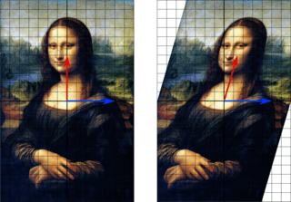
The Mona Lisa example pictured at right provides a simple illustration. Each point on the painting can be represented as a vector pointing from the center of the painting to that point. The linear transformation in this example is called a shear mapping. Points in the top half are moved to the right and points in the bottom half are moved to the left proportional to how far they are from the horizontal axis that goes through the middle of the painting. The vectors pointing to each point in the original image are therefore tilted right or left and made longer or shorter by the transformation. Notice that points along the horizontal axis do not move at all when this transformation is applied. Therefore, any vector that points directly to the right or left with no vertical component is an eigenvector of this transformation because the mapping does not change its direction. Moreover, these eigenvectors all have an eigenvalue equal to one because the mapping does not change their length, either.
Linear transformations can take many different forms, mapping vectors in a variety of vector spaces, so the eigenvectors can also take many forms. For example, the linear transformation could be a differential operator like , in which case the eigenvectors are functions called eigenfunctions that are scaled by that differential operator, such as


Alternatively, the linear transformation could take the form of an n by n matrix, in which case the eigenvectors are n by 1 matrices that are also referred to as eigenvectors. If the linear transformation is expressed in the form of an n by n matrix A, then the eigenvalue equation above for a linear transformation can be rewritten as the matrix multiplication

where the eigenvector v is an n by 1 matrix. For a matrix, eigenvalues and eigenvectors can be used to decompose the matrix, for example by diagonalizing it.
Eigenvalues and eigenvectors give rise to many closely related mathematical concepts, and the prefix eigen- is applied liberally when naming them:
- The set of all eigenvectors of a linear transformation, each paired with its corresponding eigenvalue, is called the eigensystem of that transformation.[5][6]
- The set of all eigenvectors of T corresponding to the same eigenvalue, together with the zero vector, is called an eigenspace or characteristic space of T.[7][8]
- If the set of eigenvectors of T form a basis of the domain of T, then this basis is called an eigenbasis.
History
Eigenvalues are often introduced in the context of linear algebra or matrix theory. Historically, however, they arose in the study of quadratic forms and differential equations.
In the 18th century Euler studied the rotational motion of a rigid body and discovered the importance of the principal axes.[9] Lagrange realized that the principal axes are the eigenvectors of the inertia matrix.[10] In the early 19th century, Cauchy saw how their work could be used to classify the quadric surfaces, and generalized it to arbitrary dimensions.[11] Cauchy also coined the term racine caractéristique (characteristic root) for what is now called eigenvalue; his term survives in characteristic equation.[12][13]
Fourier used the work of Laplace and Lagrange to solve the heat equation by separation of variables in his famous 1822 book Théorie analytique de la chaleur.[14] Sturm developed Fourier's ideas further and brought them to the attention of Cauchy, who combined them with his own ideas and arrived at the fact that real symmetric matrices have real eigenvalues.[11] This was extended by Hermite in 1855 to what are now called Hermitian matrices.[12] Around the same time, Brioschi proved that the eigenvalues of orthogonal matrices lie on the unit circle,[11] and Clebsch found the corresponding result for skew-symmetric matrices.[12] Finally, Weierstrass clarified an important aspect in the stability theory started by Laplace by realizing that defective matrices can cause instability.[11]
In the meantime, Liouville studied eigenvalue problems similar to those of Sturm; the discipline that grew out of their work is now called Sturm–Liouville theory.[15] Schwarz studied the first eigenvalue of Laplace's equation on general domains towards the end of the 19th century, while Poincaré studied Poisson's equation a few years later.[16]
At the start of the 20th century, Hilbert studied the eigenvalues of integral operators by viewing the operators as infinite matrices.[17] He was the first to use the German word eigen, which means "own", to denote eigenvalues and eigenvectors in 1904,[18] though he may have been following a related usage by Helmholtz. For some time, the standard term in English was "proper value", but the more distinctive term "eigenvalue" is standard today.[19]
The first numerical algorithm for computing eigenvalues and eigenvectors appeared in 1929, when Von Mises published the power method. One of the most popular methods today, the QR algorithm, was proposed independently by John G.F. Francis[20] and Vera Kublanovskaya[21] in 1961.[22]
Eigenvalues and eigenvectors of matrices
Eigenvalues and eigenvectors are often introduced to students in the context of linear algebra courses focused on matrices.[23][24] Furthermore, linear transformations can be represented using matrices,[1][2] which is especially common in numerical and computational applications.[25]

Consider n-dimensional vectors that are formed as a list of n scalars, such as the three-dimensional vectors

These vectors are said to be scalar multiples of each other, or parallel or collinear, if there is a scalar λ such that

In this case λ = −1/20.
Now consider the linear transformation of n-dimensional vectors defined by an n by n matrix A,

or

where, for each row,
- .

If it occurs that v and w are scalar multiples, that is if
-
(1)
then v is an eigenvector of the linear transformation A and the scale factor λ is the eigenvalue corresponding to that eigenvector. Equation (1) is the eigenvalue equation for the matrix A.
Equation (1) can be stated equivalently as
-
(2)

where I is the n by n identity matrix.
Eigenvalues and the characteristic polynomial
Equation (2) has a non-zero solution v if and only if the determinant of the matrix (A − λI) is zero. Therefore, the eigenvalues of A are values of λ that satisfy the equation
-
(3)

Using Leibniz' rule for the determinant, the left hand side of Equation (3) is a polynomial function of the variable λ and the degree of this polynomial is n, the order of the matrix A. Its coefficients depend on the entries of A, except that its term of degree n is always (−1)nλn. This polynomial is called the characteristic polynomial of A. Equation (3) is called the characteristic equation or the secular equation of A.
The fundamental theorem of algebra implies that the characteristic polynomial of an n by n matrix A, being a polynomial of degree n, can be factored into the product of n linear terms,
-
(4)

where each λi may be real but in general is a complex number. The numbers λ1, λ2, ... λn, which may not all have distinct values, are roots of the polynomial and are the eigenvalues of A.
As a brief example, which is described in more detail in the examples section later, consider the matrix

Taking the determinant of (M − λI), the characteristic polynomial of M is

Setting the characteristic polynomial equal to zero, it has roots at λ = 1 and λ = 3, which are the two eigenvalues of M. The eigenvectors corresponding to each eigenvalue can be found by solving for the components of v in the equation Mv = λv. In this example, the eigenvectors are any non-zero scalar multiples of

If the entries of the matrix A are all real numbers, then the coefficients of the characteristic polynomial will also be real numbers, but the eigenvalues may still have non-zero imaginary parts. The entries of the corresponding eigenvectors therefore may also have non-zero imaginary parts. Similarly, the eigenvalues may be irrational numbers even if all the entries of A are rational numbers or even if they are all integers. However, if the entries of A are all algebraic numbers, which include the rationals, the eigenvalues are complex algebraic numbers.
The non-real roots of a real polynomial with real coefficients can be grouped into pairs of complex conjugates, namely with the two members of each pair having imaginary parts that differ only in sign and the same real part. If the degree is odd, then by the intermediate value theorem at least one of the roots is real. Therefore, any real matrix with odd order has at least one real eigenvalue, whereas a real matrix with even order may not have any real eigenvalues. The eigenvectors associated with these complex eigenvalues are also complex and also appear in complex conjugate pairs.
Algebraic multiplicity
Let λi be an eigenvalue of an n by n matrix A. The algebraic multiplicity μA(λi) of the eigenvalue is its multiplicity as a root of the characteristic polynomial, that is, the largest integer k such that (λ − λi)k divides evenly that polynomial.[8][26][27]
Suppose a matrix A has dimension n and d ≤ n distinct eigenvalues. Whereas Equation (4) factors the characteristic polynomial of A into the product of n linear terms with some terms potentially repeating, the characteristic polynomial can instead be written as the product d terms each corresponding to a distinct eigenvalue and raised to the power of the algebraic multiplicity,

If d = n then the right hand side is the product of n linear terms and this is the same as Equation (4). The size of each eigenvalue's algebraic multiplicity is related to the dimension n as

If μA(λi) = 1, then λi is said to be a simple eigenvalue.[27] If μA(λi) equals the geometric multiplicity of λi, γA(λi), defined in the next section, then λi is said to be a semisimple eigenvalue.
Eigenspaces, geometric multiplicity, and the eigenbasis for matrices
Given a particular eigenvalue λ of the n by n matrix A, define the set E to be all vectors v that satisfy Equation (2),

On one hand, this set is precisely the kernel or nullspace of the matrix (A − λI). On the other hand, by definition, any non-zero vector that satisfies this condition is an eigenvector of A associated with λ. So, the set E is the union of the zero vector with the set of all eigenvectors of A associated with λ, and E equals the nullspace of (A − λI). E is called the eigenspace or characteristic space of A associated with λ.[7][8] In general λ is a complex number and the eigenvectors are complex n by 1 matrices. A property of the nullspace is that it is a linear subspace, so E is a linear subspace of ℂn.
Because the eigenspace E is a linear subspace, it is closed under addition. That is, if two vectors u and v belong to the set E, written (u,v) ∈ E, then (u + v) ∈ E or equivalently A(u + v) = λ(u + v). This can be checked using the distributive property of matrix multiplication. Similarly, because E is a linear subspace, it is closed under scalar multiplication. That is, if v ∈ E and α is a complex number, (αv) ∈ E or equivalently A(αv) = λ(αv). This can be checked by noting that multiplication of complex matrices by complex numbers is commutative. As long as u + v and αv are not zero, they are also eigenvectors of A associated with λ.
The dimension of the eigenspace E associated with λ, or equivalently the maximum number of linearly independent eigenvectors associated with λ, is referred to as the eigenvalue's geometric multiplicity γA(λ). Because E is also the nullspace of (A − λI), the geometric multiplicity of λ is the dimension of the nullspace of (A − λI), also called the nullity of (A − λI), which relates to the dimension and rank of (A - λI) as

Because of the definition of eigenvalues and eigenvectors, an eigenvalue's geometric multiplicity must be at least one, that is, each eigenvalue has at least one associated eigenvector. Furthermore, an eigenvalue's geometric multiplicity cannot exceed its algebraic multiplicity. Additionally, recall that an eigenvalue's algebraic multiplicity cannot exceed n.

The condition that γA(λ) ≤ μA(λ) can be proven by considering a particular eigenvalue ξ of A and diagonalizing the first γA(ξ) columns of A with respect to ξ's eigenvectors, described in a later section. The resulting similar matrix B is block upper triangular, with its top left block being the diagonal matrix ξIγA(ξ). As a result, the characteristic polynomial of B will have a factor of (ξ - λ)γA(ξ). The other factors of the characteristic polynomial of B are not known, so the algebraic multiplicity of ξ as an eigenvalue of B is no less than the geometric multiplicity of ξ as an eigenvalue of A. The last element of the proof is the property that similar matrices have the same characteristic polynomial.
Suppose A has d ≤ n distinct eigenvalues λ1, λ2, ..., λd, where the geometric multiplicity of λi is γA(λi). The total geometric multiplicity of A,

is the dimension of the union of all the eigenspaces of A's eigenvalues, or equivalently the maximum number of linearly independent eigenvectors of A. If γA = n, then
- The union of the eigenspaces of all of A's eigenvalues is the entire vector space ℂn
- A basis of ℂn can be formed from n linearly independent eigenvectors of A; such a basis is called an eigenbasis
- Any vector in ℂn can be written as a linear combination of eigenvectors of A
Additional properties of eigenvalues
Let A be an arbitrary n by n matrix of complex numbers with eigenvalues λ1, λ2, ..., λn. Each eigenvalue appears μA(λi) times in this list, where μA(λi) is the eigenvalue's algebraic multiplicity. The following are properties of this matrix and its eigenvalues:
- The trace of A, defined as the sum of its diagonal elements, is also the sum of all eigenvalues,

- The determinant of A is the product of all its eigenvalues,

- The eigenvalues of the kth power of A, i.e. the eigenvalues of Ak, for any positive integer k, are λ1k, λ2k, ..., λnk.
- The matrix A is invertible if and only if every eigenvalue is nonzero.
- If A is invertible, then the eigenvalues of A−1 are 1/λ1, 1/λ2, ..., 1/λn and each eigenvalue's geometric multiplicity coincides. Moreover, since the characteristic polynomial of the inverse is the reciprocal polynomial of the original, the eigenvalues share the same algebraic multiplicity.
- If A is equal to its conjugate transpose A*, or equivalently if A is Hermitian, then every eigenvalue is real. The same is true of any symmetric real matrix.
- If A is not only Hermitian but also positive-definite, positive-semidefinite, negative-definite, or negative-semidefinite, then every eigenvalue is positive, non-negative, negative, or non-positive, respectively.
- If A is unitary, every eigenvalue has absolute value |λi| = 1.
Left and right eigenvectors
Many disciplines traditionally represent vectors as matrices with a single column rather than as matrices with a single row. For that reason, the word "eigenvector" in the context of matrices almost always refers to a right eigenvector, namely a column vector that right multiples the n by n matrix A in the defining equation, Equation (1),

The eigenvalue and eigenvector problem can also be defined for row vectors that left multiply matrix A. In this formulation, the defining equation is

where κ is a scalar and u is a 1 by n matrix. Any row vector u satisfying this equation is called a left eigenvector of A and κ is its associated eigenvalue. Taking the conjugate transpose of this equation,

Comparing this equation to Equation (1), the left eigenvectors of A are the conjugate transpose of the right eigenvectors of A*. The eigenvalues of the left eigenvectors are the solution of the characteristic polynomial |A* − κ*I|=0. Because the identity matrix is Hermitian and |M*| = |M|* for a square matrix M, the eigenvalues of the left eigenvectors of A are the complex conjugates of the eigenvalues of the right eigenvectors of A. Recall that if A is a real matrix, all of its complex eigenvalues appear in complex conjugate pairs. Therefore, the eigenvalues of the left and right eigenvectors of a real matrix are the same. Similarly, if A is a real matrix, all of its complex eigenvectors also appear in complex conjugate pairs. Therefore, the left eigenvectors simplify to the transpose of the right eigenvectors of AT if A is real.
Diagonalization and the eigendecomposition
Suppose the eigenvectors of A form a basis, or equivalently A has n linearly independent eigenvectors v1, v2, ..., vn with associated eigenvalues λ1, λ2, ..., λn. The eigenvalues need not be distinct. Define a square matrix Q whose columns are the n linearly independent eigenvectors of A,

Since each column of Q is an eigenvector of A, right multiplying A by Q scales each column of Q by its associated eigenvalue,

With this in mind, define a diagonal matrix Λ where each diagonal element Λii is the eigenvalue associated with the ith column of Q. Then

Because the columns of Q are linearly independent, Q is invertible. Right multiplying both sides of the equation by Q−1,

or by instead left multiplying both sides by Q−1,

A can therefore be decomposed into a matrix composed of its eigenvectors, a diagonal matrix with its eigenvalues along the diagonal, and the inverse of the matrix of eigenvectors. This is called the eigendecomposition and it is a similarity transformation. Such a matrix A is said to be similar to the diagonal matrix Λ or diagonalizable. The matrix Q is the change of basis matrix of the similarity transformation. Essentially, the matrices A and Λ represent the same linear transformation expressed in two different bases. The eigenvectors are used as the basis when representing the linear transformation as Λ.
Conversely, suppose a matrix A is diagonalizable. Let P be a non-singular square matrix such that P−1AP is some diagonal matrix D. Left multiplying both by P, AP = PD. Each column of P must therefore be an eigenvector of A whose eigenvalue is the corresponding diagonal element of D. Since the columns of P must be linearly independent for P to be invertible, there exist n linearly independent eigenvectors of A. It then follows that the eigenvectors of A form a basis if and only if A is diagonalizable.
A matrix that is not diagonalizable is said to be defective. For defective matrices, the notion of eigenvectors generalizes to generalized eigenvectors and the diagonal matrix of eigenvalues generalizes to the Jordan normal form. Over an algebraically closed field, any matrix A has a Jordan normal form and therefore admits a basis of generalized eigenvectors and a decomposition into generalized eigenspaces.
Variational characterization
In the Hermitian case, eigenvalues can be given a variational characterization. The largest eigenvalue of is the maximum value of the quadratic form . A value of that realizes that maximum, is an eigenvector.


Matrix examples
Two-dimensional matrix example

Consider the matrix

The figure on the right shows the effect of this transformation on point coordinates in the plane. The eigenvectors v of this transformation satisfy Equation (1), and the values of λ for which the determinant of the matrix (A − λI) equals zero are the eigenvalues.
Taking the determinant to find characteristic polynomial of A,

Setting the characteristic polynomial equal to zero, it has roots at λ = 1 and λ = 3, which are the two eigenvalues of A.
For λ = 1, Equation (2) becomes,

Any non-zero vector with v1 = −v2 solves this equation. Therefore,

is an eigenvector of A corresponding to λ = 1, as is any scalar multiple of this vector.
For λ = 3, Equation (2) becomes

Any non-zero vector with v1 = v2 solves this equation. Therefore,

is an eigenvector of A corresponding to λ = 3, as is any scalar multiple of this vector.
Thus, the vectors vλ=1 and vλ=3 are eigenvectors of A associated with the eigenvalues λ = 1 and λ = 3, respectively.
Three-dimensional matrix example
Consider the matrix

The characteristic polynomial of A is
![{\displaystyle {\begin{aligned}|A-\lambda I|&=\left|{\begin{bmatrix}2&0&0\\0&3&4\\0&4&9\end{bmatrix}}-\lambda {\begin{bmatrix}1&0&0\\0&1&0\\0&0&1\end{bmatrix}}\right|\;=\;{\begin{vmatrix}2-\lambda &0&0\\0&3-\lambda &4\\0&4&9-\lambda \end{vmatrix}},\\&=(2-\lambda ){\bigl [}(3-\lambda )(9-\lambda )-16{\bigr ]}=-\lambda ^{3}+14\lambda ^{2}-35\lambda +22.\end{aligned}}}](../I/m/293ad858f6cf147cc71f1f31d040db7693dd55c9.svg)
The roots of the characteristic polynomial are 2, 1, and 11, which are the only three eigenvalues of A. These eigenvalues correspond to the eigenvectors and , or any non-zero multiple thereof.
![{\displaystyle [1\;0\;0]^{\mathrm {T} },}](../I/m/68b64d22043098396136830d084e62feb15095ae.svg)
![{\displaystyle [0\;2\;-1]^{\mathrm {T} },}](../I/m/ee7ba426be5d2c2c218956b49c0ebaf6c8f819a2.svg)
![{\displaystyle [0\;1\;2]^{\mathrm {T} }}](../I/m/807b798bac2555afb6c1cdb2a20c99e1c7d3cb53.svg)
Three-dimensional matrix example with complex eigenvalues
Consider the cyclic permutation matrix

This matrix shifts the coordinates of the vector up by one position and moves the first coordinate to the bottom. Its characteristic polynomial is 1 − λ3, whose roots are


where i = is the imaginary unit.

For the real eigenvalue λ1 = 1, any vector with three equal non-zero entries is an eigenvector. For example,

For the complex conjugate pair of imaginary eigenvalues, note that

Then

and

Therefore, the other two eigenvectors of A are complex and are and with eigenvalues λ2 and λ3, respectively. Note that the two complex eigenvectors also appear in a complex conjugate pair,
![{\displaystyle v_{\lambda _{2}}=[1\;\lambda _{2}\;\lambda _{3}]^{\mathrm {T} }}](../I/m/c9f936d252b46e5b2d5bd70ac885fcdb800eeeca.svg)
![{\displaystyle v_{\lambda _{3}}=[1\;\lambda _{3}\;\lambda _{2}]^{\mathrm {T} }}](../I/m/2d5ce3ead2bcef90216385498c3a522923ea15e6.svg)

Diagonal matrix example
Matrices with entries only along the main diagonal are called diagonal matrices. The eigenvalues of a diagonal matrix are the diagonal elements themselves. Consider the matrix

The characteristic polynomial of A is

which has the roots λ1 = 1, λ2 = 2, and λ3 = 3. These roots are the diagonal elements as well as the eigenvalues of A.
Each diagonal element corresponds to an eigenvector whose only non-zero component is in the same row as that diagonal element. In the example, the eigenvalues correspond to the eigenvectors,

respectively, as well as scalar multiples of these vectors.
Triangular matrix example
A matrix whose elements above the main diagonal are all zero is called a lower triangular matrix, while a matrix whose elements below the main diagonal are all zero is called an upper triangular matrix. As with diagonal matrices, the eigenvalues of triangular matrices are the elements of the main diagonal.
Consider the lower triangular matrix,

The characteristic polynomial of A is
which has the roots λ1 = 1, λ2 = 2, and λ3 = 3. These roots are the diagonal elements as well as the eigenvalues of A.
These eigenvalues correspond to the eigenvectors,

respectively, as well as scalar multiples of these vectors.
Matrix with repeated eigenvalues example
As in the previous example, the lower triangular matrix

has a characteristic polynomial that is the product of its diagonal elements,

The roots of this polynomial, and hence the eigenvalues, are 2 and 3. The algebraic multiplicity of each eigenvalue is 2; in other words they are both double roots. The sum of the algebraic multiplicities of each distinct eigenvalue is μA = 4 = n, the order of the characteristic polynomial and the dimension of A.
On the other hand, the geometric multiplicity of the eigenvalue 2 is only 1, because its eigenspace is spanned by just one vector [0 1 -1 1]T and is therefore 1-dimensional. Similarly, the geometric multiplicity of the eigenvalue 3 is 1 because its eigenspace is spanned by just one vector [0 0 0 1]T. The total geometric multiplicity γA is 2, which is the smallest it could be for a matrix with two distinct eigenvalues. Geometric multiplicities are defined in a later section.
Eigenvalues and eigenfunctions of differential operators
The definitions of eigenvalue and eigenvectors of a linear transformation T remains valid even if the underlying vector space is an infinite-dimensional Hilbert or Banach space. A widely used class of linear transformations acting on infinite-dimensional spaces are the differential operators on function spaces. Let D be a linear differential operator on the space C∞ of infinitely differentiable real functions of a real argument t. The eigenvalue equation for D is the differential equation

The functions that satisfy this equation are eigenvectors of D and are commonly called eigenfunctions.
Derivative operator example
Consider the derivative operator with eigenvalue equation


This differential equation can be solved by multiplying both sides by dt/f(t) and integrating. Its solution, the exponential function

is the eigenfunction of the derivative operator. Note that in this case the eigenfunction is itself a function of its associated eigenvalue. In particular, note that for λ = 0 the eigenfunction f(t) is a constant.
The main eigenfunction article gives other examples.
General definition
The concept of eigenvalues and eigenvectors extends naturally to arbitrary linear transformations on arbitrary vector spaces. Let V be any vector space over some field K of scalars, and let T be a linear transformation mapping V into V,

We say that a non-zero vector v ∈ V is an eigenvector of T if and only if there exists a scalar λ ∈ K such that
-
(5)

This equation is called the eigenvalue equation for T, and the scalar λ is the eigenvalue of T corresponding to the eigenvector v. Note that T(v) is the result of applying the transformation T to the vector v, while λv is the product of the scalar λ with v.[33]
Eigenspaces, geometric multiplicity, and the eigenbasis
Given an eigenvalue λ, consider the set

which is the union of the zero vector with the set of all eigenvectors associated with λ. E is called the eigenspace or characteristic space of T associated with λ.
By definition of a linear transformation,

for (x,y) ∈ V and α ∈ K. Therefore, if u and v are eigenvectors of T associated with eigenvalue λ, namely (u,v) ∈ E, then

So, both u + v and αv are either zero or eigenvectors of T associated with λ, namely (u+v,αv) ∈ E, and E is closed under addition and scalar multiplication. The eigenspace E associated with λ is therefore a linear subspace of V.[8][34][35] If that subspace has dimension 1, it is sometimes called an eigenline.[36]
The geometric multiplicity γT(λ) of an eigenvalue λ is the dimension of the eigenspace associated with λ, i.e., the maximum number of linearly independent eigenvectors associated with that eigenvalue.[8][27] By the definition of eigenvalues and eigenvectors, γT(λ) ≥ 1 because every eigenvalue has at least one eigenvector.
The eigenspaces of T always form a direct sum. As a consequence, eigenvectors of different eigenvalues are always linearly independent. Therefore, the sum of the dimensions of the eigenspaces cannot exceed the dimension n of the vector space on which T operates, and there cannot be more than n distinct eigenvalues.[37]
Any subspace spanned by eigenvectors of T is an invariant subspace of T, and the restriction of T to such a subspace is diagonalizable. Moreover, if the entire vector space V can be spanned by the eigenvectors of T, or equivalently if the direct sum of the eigenspaces associated with all the eigenvalues of T is the entire vector space V, then a basis of V called an eigenbasis can be formed from linearly independent eigenvectors of T. When T admits an eigenbasis, T is diagonalizable.
Zero vector as an eigenvector
While the definition of an eigenvector used in this article excludes the zero vector, it is possible to define eigenvalues and eigenvectors such that the zero vector is an eigenvector.[38]
Consider again the eigenvalue equation, Equation (5). Define an eigenvalue to be any scalar λ ∈ K such that there exists a non-zero vector v ∈ V satisfying Equation (5). It is important that this version of the definition of an eigenvalue specify that the vector be non-zero, otherwise by this definition the zero vector would allow any scalar in K to be an eigenvalue. Define an eigenvector v associated with the eigenvalue λ to be any vector that, given λ, satisfies Equation (5). Given the eigenvalue, the zero vector is among the vectors that satisfy Equation (5), so the zero vector is included among the eigenvectors by this alternate definition.
Spectral theory
If λ is an eigenvalue of T, then the operator (T − λI) is not one-to-one, and therefore its inverse (T − λI)−1 does not exist. The converse is true for finite-dimensional vector spaces, but not for infinite-dimensional vector spaces. In general, the operator (T − λI) may not have an inverse even if λ is not an eigenvalue.
For this reason, in functional analysis eigenvalues can be generalized to the spectrum of a linear operator T as the set of all scalars λ for which the operator (T − λI) has no bounded inverse. The spectrum of an operator always contains all its eigenvalues but is not limited to them.
Associative algebras and representation theory
One can generalize the algebraic object that is acting on the vector space, replacing a single operator acting on a vector space with an algebra representation – an associative algebra acting on a module. The study of such actions is the field of representation theory.
The representation-theoretical concept of weight is an analog of eigenvalues, while weight vectors and weight spaces are the analogs of eigenvectors and eigenspaces, respectively.
Dynamic equations
The simplest difference equations have the form

The solution of this equation for x in terms of t is found by using its characteristic equation

which can be found by stacking into matrix form a set of equations consisting of the above difference equation and the k–1 equations giving a k-dimensional system of the first order in the stacked variable vector in terms of its once-lagged value, and taking the characteristic equation of this system's matrix. This equation gives k characteristic roots for use in the solution equation

![[x_{t},\dots ,x_{t-k+1}]](../I/m/4d1478d7f39b38a62daa2350e73367d9a6035290.svg)


A similar procedure is used for solving a differential equation of the form

Calculation
Eigenvalues
The eigenvalues of a matrix can be determined by finding the roots of the characteristic polynomial. Explicit algebraic formulas for the roots of a polynomial exist only if the degree is 4 or less. According to the Abel–Ruffini theorem there is no general, explicit and exact algebraic formula for the roots of a polynomial with degree 5 or more.


It turns out that any polynomial with degree is the characteristic polynomial of some companion matrix of order . Therefore, for matrices of order 5 or more, the eigenvalues and eigenvectors cannot be obtained by an explicit algebraic formula, and must therefore be computed by approximate numerical methods.
In theory, the coefficients of the characteristic polynomial can be computed exactly, since they are sums of products of matrix elements; and there are algorithms that can find all the roots of a polynomial of arbitrary degree to any required accuracy.[39] However, this approach is not viable in practice because the coefficients would be contaminated by unavoidable round-off errors, and the roots of a polynomial can be an extremely sensitive function of the coefficients (as exemplified by Wilkinson's polynomial).[39]
Efficient, accurate methods to compute eigenvalues and eigenvectors of arbitrary matrices were not known until the advent of the QR algorithm in 1961. [39] Combining the Householder transformation with the LU decomposition results in an algorithm with better convergence than the QR algorithm. For large Hermitian sparse matrices, the Lanczos algorithm is one example of an efficient iterative method to compute eigenvalues and eigenvectors, among several other possibilities.[39]
Eigenvectors
Once the (exact) value of an eigenvalue is known, the corresponding eigenvectors can be found by finding non-zero solutions of the eigenvalue equation, that becomes a system of linear equations with known coefficients. For example, once it is known that 6 is an eigenvalue of the matrix

we can find its eigenvectors by solving the equation , that is


This matrix equation is equivalent to two linear equations
- that is


Both equations reduce to the single linear equation . Therefore, any vector of the form , for any non-zero real number , is an eigenvector of with eigenvalue .

![[a,2a]'](../I/m/9f52352fcfea5013455a3ab777c0dc9547fd610b.svg)


The matrix above has another eigenvalue . A similar calculation shows that the corresponding eigenvectors are the non-zero solutions of , that is, any vector of the form , for any non-zero real number .


![[b,-3b]'](../I/m/db10113cbb02112cf6b02e95f7f12438b79aa34e.svg)

Some numeric methods that compute the eigenvalues of a matrix also determine a set of corresponding eigenvectors as a by-product of the computation.
Applications
Eigenvalues of geometric transformations
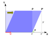
The following table presents some example transformations in the plane along with their 2×2 matrices, eigenvalues, and eigenvectors.
| scaling | unequal scaling | rotation | horizontal shear | hyperbolic rotation | |
| illustration |  |
 |
 |
 |
 |
| matrix | |
|
|
|
|
| characteristic polynomial |
|||||
| eigenvalues | , | ||||
| algebraic multipl. |
|||||
| geometric multipl. |
|||||
| eigenvectors | All non-zero vectors |


Note that the characteristic equation for a rotation is a quadratic equation with discriminant , which is a negative number whenever is not an integer multiple of 180°. Therefore, except for these special cases, the two eigenvalues are complex numbers, ; and all eigenvectors have non-real entries. Indeed, except for those special cases, a rotation changes the direction of every nonzero vector in the plane.


A linear transformation that takes a square to a rectangle of the same area (a squeeze mapping) has reciprocal eigenvalues.
Schrödinger equation


An example of an eigenvalue equation where the transformation is represented in terms of a differential operator is the time-independent Schrödinger equation in quantum mechanics:


where , the Hamiltonian, is a second-order differential operator and , the wavefunction, is one of its eigenfunctions corresponding to the eigenvalue , interpreted as its energy.


However, in the case where one is interested only in the bound state solutions of the Schrödinger equation, one looks for within the space of square integrable functions. Since this space is a Hilbert space with a well-defined scalar product, one can introduce a basis set in which and can be represented as a one-dimensional array (i.e., a vector) and a matrix respectively. This allows one to represent the Schrödinger equation in a matrix form.
The bra–ket notation is often used in this context. A vector, which represents a state of the system, in the Hilbert space of square integrable functions is represented by . In this notation, the Schrödinger equation is:


where is an eigenstate of and represents the eigenvalue. is an observable self adjoint operator, the infinite-dimensional analog of Hermitian matrices. As in the matrix case, in the equation above is understood to be the vector obtained by application of the transformation to .

Molecular orbitals
In quantum mechanics, and in particular in atomic and molecular physics, within the Hartree–Fock theory, the atomic and molecular orbitals can be defined by the eigenvectors of the Fock operator. The corresponding eigenvalues are interpreted as ionization potentials via Koopmans' theorem. In this case, the term eigenvector is used in a somewhat more general meaning, since the Fock operator is explicitly dependent on the orbitals and their eigenvalues. Thus, if one wants to underline this aspect, one speaks of nonlinear eigenvalue problems. Such equations are usually solved by an iteration procedure, called in this case self-consistent field method. In quantum chemistry, one often represents the Hartree–Fock equation in a non-orthogonal basis set. This particular representation is a generalized eigenvalue problem called Roothaan equations.
Geology and glaciology
In geology, especially in the study of glacial till, eigenvectors and eigenvalues are used as a method by which a mass of information of a clast fabric's constituents' orientation and dip can be summarized in a 3-D space by six numbers. In the field, a geologist may collect such data for hundreds or thousands of clasts in a soil sample, which can only be compared graphically such as in a Tri-Plot (Sneed and Folk) diagram,[40][41] or as a Stereonet on a Wulff Net.[42]
The output for the orientation tensor is in the three orthogonal (perpendicular) axes of space. The three eigenvectors are ordered by their eigenvalues ;[43] then is the primary orientation/dip of clast, is the secondary and is the tertiary, in terms of strength. The clast orientation is defined as the direction of the eigenvector, on a compass rose of 360°. Dip is measured as the eigenvalue, the modulus of the tensor: this is valued from 0° (no dip) to 90° (vertical). The relative values of , , and are dictated by the nature of the sediment's fabric. If , the fabric is said to be isotropic. If , the fabric is said to be planar. If , the fabric is said to be linear.[44]


Principal component analysis
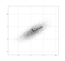


The eigendecomposition of a symmetric positive semidefinite (PSD) matrix yields an orthogonal basis of eigenvectors, each of which has a nonnegative eigenvalue. The orthogonal decomposition of a PSD matrix is used in multivariate analysis, where the sample covariance matrices are PSD. This orthogonal decomposition is called principal components analysis (PCA) in statistics. PCA studies linear relations among variables. PCA is performed on the covariance matrix or the correlation matrix (in which each variable is scaled to have its sample variance equal to one). For the covariance or correlation matrix, the eigenvectors correspond to principal components and the eigenvalues to the variance explained by the principal components. Principal component analysis of the correlation matrix provides an orthonormal eigen-basis for the space of the observed data: In this basis, the largest eigenvalues correspond to the principal components that are associated with most of the covariability among a number of observed data.
Principal component analysis is used to study large data sets, such as those encountered in bioinformatics, data mining, chemical research, psychology, and in marketing. PCA is popular especially in psychology, in the field of psychometrics. In Q methodology, the eigenvalues of the correlation matrix determine the Q-methodologist's judgment of practical significance (which differs from the statistical significance of hypothesis testing; cf. criteria for determining the number of factors). More generally, principal component analysis can be used as a method of factor analysis in structural equation modeling.
Vibration analysis

Eigenvalue problems occur naturally in the vibration analysis of mechanical structures with many degrees of freedom. The eigenvalues are the natural frequencies (or eigenfrequencies) of vibration, and the eigenvectors are the shapes of these vibrational modes. In particular, undamped vibration is governed by

or

that is, acceleration is proportional to position (i.e., we expect to be sinusoidal in time).
In dimensions, becomes a mass matrix and a stiffness matrix. Admissible solutions are then a linear combination of solutions to the generalized eigenvalue problem


where is the eigenvalue and is the (imaginary) angular frequency. Note that the principal vibration modes are different from the principal compliance modes, which are the eigenvectors of alone. Furthermore, damped vibration, governed by


leads to a so-called quadratic eigenvalue problem,

This can be reduced to a generalized eigenvalue problem by clever use of algebra at the cost of solving a larger system.
The orthogonality properties of the eigenvectors allows decoupling of the differential equations so that the system can be represented as linear summation of the eigenvectors. The eigenvalue problem of complex structures is often solved using finite element analysis, but neatly generalize the solution to scalar-valued vibration problems.
Eigenfaces
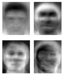
In image processing, processed images of faces can be seen as vectors whose components are the brightnesses of each pixel.[45] The dimension of this vector space is the number of pixels. The eigenvectors of the covariance matrix associated with a large set of normalized pictures of faces are called eigenfaces; this is an example of principal components analysis. They are very useful for expressing any face image as a linear combination of some of them. In the facial recognition branch of biometrics, eigenfaces provide a means of applying data compression to faces for identification purposes. Research related to eigen vision systems determining hand gestures has also been made.
Similar to this concept, eigenvoices represent the general direction of variability in human pronunciations of a particular utterance, such as a word in a language. Based on a linear combination of such eigenvoices, a new voice pronunciation of the word can be constructed. These concepts have been found useful in automatic speech recognition systems for speaker adaptation.
Tensor of moment of inertia
In mechanics, the eigenvectors of the moment of inertia tensor define the principal axes of a rigid body. The tensor of moment of inertia is a key quantity required to determine the rotation of a rigid body around its center of mass.
Stress tensor
In solid mechanics, the stress tensor is symmetric and so can be decomposed into a diagonal tensor with the eigenvalues on the diagonal and eigenvectors as a basis. Because it is diagonal, in this orientation, the stress tensor has no shear components; the components it does have are the principal components.
Graphs
In spectral graph theory, an eigenvalue of a graph is defined as an eigenvalue of the graph's adjacency matrix , or (increasingly) of the graph's Laplacian matrix due to its Discrete Laplace operator, which is either (sometimes called the combinatorial Laplacian) or (sometimes called the normalized Laplacian), where is a diagonal matrix with equal to the degree of vertex , and in , the th diagonal entry is . The th principal eigenvector of a graph is defined as either the eigenvector corresponding to the th largest or th smallest eigenvalue of the Laplacian. The first principal eigenvector of the graph is also referred to merely as the principal eigenvector.


The principal eigenvector is used to measure the centrality of its vertices. An example is Google's PageRank algorithm. The principal eigenvector of a modified adjacency matrix of the World Wide Web graph gives the page ranks as its components. This vector corresponds to the stationary distribution of the Markov chain represented by the row-normalized adjacency matrix; however, the adjacency matrix must first be modified to ensure a stationary distribution exists. The second smallest eigenvector can be used to partition the graph into clusters, via spectral clustering. Other methods are also available for clustering.
Basic reproduction number
The basic reproduction number () is a fundamental number in the study of how infectious diseases spread. If one infectious person is put into a population of completely susceptible people, then is the average number of people that one typical infectious person will infect. The generation time of an infection is the time, , from one person becoming infected to the next person becoming infected. In a heterogeneous population, the next generation matrix defines how many people in the population will become infected after time has passed. is then the largest eigenvalue of the next generation matrix.[46][47]


See also
- Antieigenvalue theory
- Eigenplane
- Eigenvalue algorithm
- Introduction to eigenstates
- Jordan normal form
- List of numerical analysis software
- Nonlinear eigenproblem
- Quadratic eigenvalue problem
- Singular value
Notes
- 1 2 Herstein (1964, pp. 228,229)
- 1 2 Nering (1970, p. 38)
- ↑ Burden & Faires (1993, p. 401)
- ↑ Betteridge (1965)
- ↑ Press (2007, p. 536)
- ↑ Wolfram Research, Inc. (2010) Eigenvector. Accessed on 2016-04-01.
- 1 2 Anton (1987, pp. 305,307)
- 1 2 3 4 5 Nering (1970, p. 107)
- ↑ Note:
- In 1751, Leonhard Euler proved that any body has a principal axis of rotation: Leonhard Euler (presented: October 1751 ; published: 1760) "Du mouvement d'un corps solide quelconque lorsqu'il tourne autour d'un axe mobile" (On the movement of any solid body while it rotates around a moving axis), Histoire de l'Académie royale des sciences et des belles lettres de Berlin, pp.176-227. On p. 212, Euler proves that any body contains a principal axis of rotation: "Théorem. 44. De quelque figure que soit le corps, on y peut toujours assigner un tel axe, qui passe par son centre de gravité, autour duquel le corps peut tourner librement & d'un mouvement uniforme." (Theorem. 44. Whatever be the shape of the body, one can always assign to it such an axis, which passes through its center of gravity, around which it can rotate freely and with a uniform motion.)
- In 1755, Johann Andreas Segner proved that any body has three principal axes of rotation: Johann Andreas Segner, Specimen theoriae turbinum [Essay on the theory of tops (i.e., rotating bodies)] ( Halle ("Halae"), (Germany) : Gebauer, 1755). On p. XXVIIII (i.e., 29), Segner derives a third-degree equation in t, which proves that a body has three principal axes of rotation. He then states (on the same page): "Non autem repugnat tres esse eiusmodi positiones plani HM, quia in aequatione cubica radices tres esse possunt, et tres tangentis t valores." (However, it is not inconsistent [that there] be three such positions of the plane HM, because in cubic equations, [there] can be three roots, and three values of the tangent t.)
- The relevant passage of Segner's work was discussed briefly by Arthur Cayley. See: A. Cayley (1862) "Report on the progress of the solution of certain special problems of dynamics," Report of the Thirty-second meeting of the British Association for the Advancement of Science; held at Cambridge in October 1862, 32 : 184-252 ; see especially pages 225-226.
- ↑ See Hawkins 1975, §2
- 1 2 3 4 See Hawkins 1975, §3
- 1 2 3 See Kline 1972, pp. 807–808
- ↑ Augustin Cauchy (1839) "Mémoire sur l'intégration des équations linéaires" (Memoir on the integration of linear equations), Comptes rendus, 8 : 827-830, 845-865, 889-907, 931-937. From p. 827: "On sait d'ailleurs qu'en suivant la méthode de Lagrange, on obtient pour valeur générale de la variable prinicipale une fonction dans laquelle entrent avec la variable principale les racines d'une certaine équation que j'appellerai l'équation caractéristique, le degré de cette équation étant précisément l'order de l'équation différentielle qu'il s'agit d'intégrer." (On knows, moreover, that by following Lagrange's method, one obtains for the general value of the principal variable a function in which there appear, together with the principal variable, the roots of a certain equation that I will call the "characteristic equation", the degree of this equation being precisely the order of the differential equation that must be integrated.)
- ↑ See Kline 1972, p. 673
- ↑ See Kline 1972, pp. 715–716
- ↑ See Kline 1972, pp. 706–707
- ↑ See Kline 1972, p. 1063
- ↑ See:
- David Hilbert (1904) "Grundzüge einer allgemeinen Theorie der linearen Integralgleichungen. (Erste Mitteilung)" (Fundamentals of a general theory of linear integral equations. (First report)), Nachrichten von der Gesellschaft der Wissenschaften zu Göttingen, Mathematisch-Physikalische Klasse (News of the Philosophical Society at Göttingen, mathematical-physical section), pp. 49-91. From page 51: "Insbesondere in dieser ersten Mitteilung gelange ich zu Formeln, die die Entwickelung einer willkürlichen Funktion nach gewissen ausgezeichneten Funktionen, die ich Eigenfunktionen nenne, liefern: … (In particular, in this first report I arrive at formulas that provide the [series] development of an arbitrary function in terms of some distinctive functions, which I call eigenfunctions: … ) Later on the same page: "Dieser Erfolg ist wesentlich durch den Umstand bedingt, daß ich nicht, wie es bisher geschah, in erster Linie auf den Beweis für die Existenz der Eigenwerte ausgehe, … " (This success is mainly attributable to the fact that I do not, as it has happened until now, first of all aim at a proof of the existence of eigenvalues, … )
- For the origin and evolution of the terms eigenvalue, characteristic value, etc., see: Earliest Known Uses of Some of the Words of Mathematics (E)
- ↑ See Aldrich 2006
- ↑ Francis, J. G. F. (1961), "The QR Transformation, I (part 1)", The Computer Journal, 4 (3): 265–271, doi:10.1093/comjnl/4.3.265 and Francis, J. G. F. (1962), "The QR Transformation, II (part 2)", The Computer Journal, 4 (4): 332–345, doi:10.1093/comjnl/4.4.332
- ↑ Kublanovskaya, Vera N. (1961), "On some algorithms for the solution of the complete eigenvalue problem", USSR Computational Mathematics and Mathematical Physics, 3: 637–657. Also published in: "О некоторых алгорифмах для решения полной проблемы собственных значений" [On certain algorithms for the solution of the complete eigenvalue problem], Журнал вычислительной математики и математической физики (Journal of Computational Mathematics and Mathematical Physics), 1 (4): 555–570, 1961
- ↑ See Golub & van Loan 1996, §7.3; Meyer 2000, §7.3
- ↑ Cornell University Department of Mathematics (2016) Lower-Level Courses for Freshmen and Sophomores. Accessed on 2016-03-27.
- ↑ University of Michigan Mathematics (2016) Math Course Catalogue. Accessed on 2016-03-27.
- ↑ Press (2007, pp. 38)
- ↑ Fraleigh (1976, p. 358)
- 1 2 3 Golub & Van Loan (1996, p. 316)
- 1 2 Beauregard & Fraleigh (1973, p. 307)
- ↑ Herstein (1964, p. 272)
- ↑ Nering (1970, pp. 115–116)
- ↑ Herstein (1964, p. 290)
- ↑ Nering (1970, p. 116)
- ↑ See Korn & Korn 2000, Section 14.3.5a; Friedberg, Insel & Spence 1989, p. 217
- ↑ Shilov 1977, p. 109
- ↑ Lemma for the eigenspace
- ↑ Schaum's Easy Outline of Linear Algebra, p. 111
- ↑ For a proof of this lemma, see Roman 2008, Theorem 8.2 on p. 186; Shilov 1977, p. 109; Hefferon 2001, p. 364; Beezer 2006, Theorem EDELI on p. 469; and Lemma for linear independence of eigenvectors
- ↑ Axler, Sheldon, "Ch. 5", Linear Algebra Done Right (2nd ed.), p. 77
- 1 2 3 4 Trefethen, Lloyd N.; Bau, David (1997), Numerical Linear Algebra, SIAM
- ↑ Graham, D.; Midgley, N. (2000), "Graphical representation of particle shape using triangular diagrams: an Excel spreadsheet method", Earth Surface Processes and Landforms, 25 (13): 1473–1477, Bibcode:2000ESPL...25.1473G, doi:10.1002/1096-9837(200012)25:13<1473::AID-ESP158>3.0.CO;2-C
- ↑ Sneed, E. D.; Folk, R. L. (1958), "Pebbles in the lower Colorado River, Texas, a study of particle morphogenesis", Journal of Geology, 66 (2): 114–150, Bibcode:1958JG.....66..114S, doi:10.1086/626490
- ↑ Knox-Robinson, C.; Gardoll, Stephen J. (1998), "GIS-stereoplot: an interactive stereonet plotting module for ArcView 3.0 geographic information system", Computers & Geosciences, 24 (3): 243, Bibcode:1998CG.....24..243K, doi:10.1016/S0098-3004(97)00122-2
- ↑ Stereo32 software
- ↑ Benn, D.; Evans, D. (2004), A Practical Guide to the study of Glacial Sediments, London: Arnold, pp. 103–107
- ↑ Xirouhakis, A.; Votsis, G.; Delopoulus, A. (2004), Estimation of 3D motion and structure of human faces (PDF), National Technical University of Athens
- ↑ Diekmann O, Heesterbeek JA, Metz JA (1990), "On the definition and the computation of the basic reproduction ratio R0 in models for infectious diseases in heterogeneous populations", Journal of Mathematical Biology, 28 (4): 365–382, doi:10.1007/BF00178324, PMID 2117040
- ↑ Odo Diekmann; J. A. P. Heesterbeek (2000), Mathematical epidemiology of infectious diseases, Wiley series in mathematical and computational biology, West Sussex, England: John Wiley & Sons
References
- Akivis, Max A.; Goldberg, Vladislav V. (1969), Tensor calculus, Russian, Science Publishers, Moscow
- Aldrich, John (2006), "Eigenvalue, eigenfunction, eigenvector, and related terms", in Jeff Miller (Editor), Earliest Known Uses of Some of the Words of Mathematics, retrieved 2006-08-22
- Alexandrov, Pavel S. (1968), Lecture notes in analytical geometry, Russian, Science Publishers, Moscow
- Anton, Howard (1987), Elementary Linear Algebra (5th ed.), New York: Wiley, ISBN 0-471-84819-0
- Beauregard, Raymond A.; Fraleigh, John B. (1973), A First Course In Linear Algebra: with Optional Introduction to Groups, Rings, and Fields, Boston: Houghton Mifflin Co., ISBN 0-395-14017-X
- Beezer, Robert A. (2006), A first course in linear algebra, Free online book under GNU licence, University of Puget Sound
- Betteridge, Harold T. (1965), The New Cassell's German Dictionary, New York: Funk & Wagnall, LCCN 58-7924
- Bowen, Ray M.; Wang, Chao-Cheng (1980), Linear and multilinear algebra, Plenum Press, New York, ISBN 0-306-37508-7
- Brown, Maureen (October 2004), Illuminating Patterns of Perception: An Overview of Q Methodology
- Burden, Richard L.; Faires, J. Douglas (1993), Numerical Analysis (5th ed.), Boston: Prindle, Weber and Schmidt, ISBN 0-534-93219-3
- Carter, Tamara A.; Tapia, Richard A.; Papaconstantinou, Anne, Linear Algebra: An Introduction to Linear Algebra for Pre-Calculus Students, Rice University, Online Edition, retrieved 2008-02-19
- Cohen-Tannoudji, Claude (1977), "Chapter II. The mathematical tools of quantum mechanics", Quantum mechanics, John Wiley & Sons, ISBN 0-471-16432-1
- Curtis, Charles W. (1999), Linear Algebra: An Introductory Approach (4th ed.), Springer, ISBN 0-387-90992-3
- Demmel, James W. (1997), Applied numerical linear algebra, SIAM, ISBN 0-89871-389-7
- Fraleigh, John B. (1976), A First Course In Abstract Algebra (2nd ed.), Reading: Addison-Wesley, ISBN 0-201-01984-1
- Fraleigh, John B.; Beauregard, Raymond A. (1995), Linear algebra (3rd ed.), Addison-Wesley Publishing Company, ISBN 0-201-83999-7
- Friedberg, Stephen H.; Insel, Arnold J.; Spence, Lawrence E. (1989), Linear algebra (2nd ed.), Englewood Cliffs, New Jersey 07632: Prentice Hall, ISBN 0-13-537102-3
- Gelfand, I. M. (1971), Lecture notes in linear algebra, Russian, Science Publishers, Moscow
- Gohberg, Israel; Lancaster, Peter; Rodman, Leiba (2005), Indefinite linear algebra and applications, Basel-Boston-Berlin: Birkhäuser Verlag, ISBN 3-7643-7349-0
- Golub, Gene F.; van der Vorst, Henk A. (2000), "Eigenvalue computation in the 20th century", Journal of Computational and Applied Mathematics, 123: 35–65, Bibcode:2000JCoAM.123...35G, doi:10.1016/S0377-0427(00)00413-1
- Golub, Gene H.; Van Loan, Charles F. (1996), Matrix computations (3rd ed.), Johns Hopkins University Press, Baltimore, Maryland, ISBN 978-0-8018-5414-9
- Greub, Werner H. (1975), Linear Algebra (4th ed.), Springer-Verlag, New York, ISBN 0-387-90110-8
- Halmos, Paul R. (1987), Finite-dimensional vector spaces (8th ed.), New York: Springer-Verlag, ISBN 0-387-90093-4
- Hawkins, T. (1975), "Cauchy and the spectral theory of matrices", Historia Mathematica, 2: 1–29, doi:10.1016/0315-0860(75)90032-4
- Hefferon, Jim (2001), Linear Algebra, Online book, St Michael's College, Colchester, Vermont, USA
- Herstein, I. N. (1964), Topics In Algebra, Waltham: Blaisdell Publishing Company, ISBN 978-1114541016
- Horn, Roger A.; Johnson, Charles F. (1985), Matrix analysis, Cambridge University Press, ISBN 0-521-30586-1
- Kline, Morris (1972), Mathematical thought from ancient to modern times, Oxford University Press, ISBN 0-19-501496-0
- Korn, Granino A.; Korn, Theresa M. (2000), "Mathematical Handbook for Scientists and Engineers: Definitions, Theorems, and Formulas for Reference and Review", New York: McGraw-Hill (2nd Revised ed.), Dover Publications, Bibcode:1968mhse.book.....K, ISBN 0-486-41147-8
- Kuttler, Kenneth (2007), An introduction to linear algebra (PDF), Online e-book in PDF format, Brigham Young University
- Lancaster, P. (1973), Matrix theory, Russian, Moscow, Russia: Science Publishers
- Larson, Ron; Edwards, Bruce H. (2003), Elementary linear algebra (5th ed.), Houghton Mifflin Company, ISBN 0-618-33567-6
- Lipschutz, Seymour (1991), Schaum's outline of theory and problems of linear algebra, Schaum's outline series (2nd ed.), New York: McGraw-Hill Companies, ISBN 0-07-038007-4
- Meyer, Carl D. (2000), Matrix analysis and applied linear algebra, Society for Industrial and Applied Mathematics (SIAM), Philadelphia, ISBN 978-0-89871-454-8
- Nering, Evar D. (1970), Linear Algebra and Matrix Theory (2nd ed.), New York: Wiley, LCCN 76091646
- (Russian)Pigolkina, T. S.; Shulman, V. S. (1977). "Eigenvalue". In Vinogradov, I. M. Mathematical Encyclopedia. 5. Moscow: Soviet Encyclopedia.
- Press, William H.; Teukolsky, Saul A.; Vetterling, William T.; Flannery, Brian P. (2007), Numerical Recipes: The Art of Scientific Computing (3rd ed.), ISBN 9780521880688
- Roman, Steven (2008), Advanced linear algebra (3rd ed.), New York: Springer Science + Business Media, LLC, ISBN 978-0-387-72828-5
- Sharipov, Ruslan A. (1996), Course of Linear Algebra and Multidimensional Geometry: the textbook, arXiv:math/0405323
 , Bibcode:2004math......5323S, ISBN 5-7477-0099-5
 - Shilov, Georgi E. (1977), Linear algebra, Translated and edited by Richard A. Silverman, New York: Dover Publications, ISBN 0-486-63518-X
- Shores, Thomas S. (2007), Applied linear algebra and matrix analysis, Springer Science+Business Media, LLC, ISBN 0-387-33194-8
- Strang, Gilbert (1993), Introduction to linear algebra, Wellesley-Cambridge Press, Wellesley, Massachusetts, ISBN 0-9614088-5-5
- Strang, Gilbert (2006), Linear algebra and its applications, Thomson, Brooks/Cole, Belmont, California, ISBN 0-03-010567-6
External links
| The Wikibook Linear Algebra has a page on the topic of: Eigenvalues and Eigenvectors |
| The Wikibook The Book of Mathematical Proofs has a page on the topic of: Algebra/Linear Transformations |
- What are Eigen Values? – non-technical introduction from PhysLink.com's "Ask the Experts"
- Eigen Values and Eigen Vectors Numerical Examples – Tutorial and Interactive Program from Revoledu.
- Introduction to Eigen Vectors and Eigen Values – lecture from Khan Academy
- Hill, Roger (2009). "λ – Eigenvalues". Sixty Symbols. Brady Haran for the University of Nottingham.
- "A Beginner's Guide to Eigenvectors". Deeplearning4j. 2015.
Theory
- Hazewinkel, Michiel, ed. (2001), "Eigen value", Encyclopedia of Mathematics, Springer, ISBN 978-1-55608-010-4
- Hazewinkel, Michiel, ed. (2001), "Eigen vector", Encyclopedia of Mathematics, Springer, ISBN 978-1-55608-010-4
- "Eigenvalue (of a matrix)". PlanetMath.
- Eigenvector – Wolfram MathWorld
- Eigen Vector Examination working applet
- Same Eigen Vector Examination as above in a Flash demo with sound
- Computation of Eigenvalues
- Numerical solution of eigenvalue problems Edited by Zhaojun Bai, James Demmel, Jack Dongarra, Axel Ruhe, and Henk van der Vorst
- Eigenvalues and Eigenvectors on the Ask Dr. Math forums: ,
Demonstration applets
- Java applet about eigenvectors in the real plane
- Wolfram Language functionality for Eigenvalues, Eigenvectors and Eigensystems