Multidimensional scaling
Multidimensional scaling (MDS) is a means of visualizing the level of similarity of individual cases of a dataset. It refers to a set of related ordination techniques used in information visualization, in particular to display the information contained in a distance matrix. An MDS algorithm aims to place each object in N-dimensional space such that the between-object distances are preserved as well as possible. Each object is then assigned coordinates in each of the N dimensions. The number of dimensions of an MDS plot N can exceed 2 and is specified a priori. Choosing N=2 optimizes the object locations for a two-dimensional scatterplot.[1]
Types
MDS algorithms fall into a taxonomy, depending on the meaning of the input matrix:
Classical multidimensional scaling
It is also known as Principal Coordinates Analysis, Torgerson Scaling or Torgerson–Gower scaling. It takes an input matrix giving dissimilarities between pairs of items and outputs a coordinate matrix whose configuration minimizes a loss function called strain:[1] For example, given the aerial distances between many cities in a matrix , where is the distance between the coordinates of and city, given by . Now, you want to find the coordinates of the cities. This problem is addressed in classical MDS.
![{\textstyle D=[d_{ij}]}](../I/m/f4a19ec41d512d847550da4ad3bef8a9d87e1498.svg)


- General forms of loss functions called Stress in distance MDS and Strain in classical MDS. The strain is given by:
, where are the terms of the matrix defined on step 2 of the following algorithm.
- Steps of a Classical MDS algorithm:
- Classical MDS uses the fact that the coordinate matrix can be derived by eigenvalue decomposition from . And the matrix can be computed from proximity matrix by using double centering.[2]
- Set up the squared proximity matrix
- Apply double centering: using the centering matrix , where is the number of objects.
- Determine the largest eigenvalues and corresponding eigenvectors of (where is the number of dimensions desired for the output).
- Now, , where is the matrix of eigenvectors and is the diagonal matrix of eigenvalues of .
- Classical MDS assumes Euclidean distances. So this is not applicable for direct dissimilarity ratings.


![{\textstyle D^{(2)}=[d_{ij}^{2}]}](../I/m/0b27ab659b07dca79ef150ed7ef1bfb4259f6a08.svg)


Metric multidimensional scaling
It is a superset of classical MDS that generalizes the optimization procedure to a variety of loss functions and input matrices of known distances with weights and so on. A useful loss function in this context is called stress, which is often minimized using a procedure called stress majorization. Metric MDS minimizes the cost function called “Stress” which is a residual sum of squares:

: or,

- Metric scaling uses a power transformation with a user-controlled exponent : and for distance. In classical scaling . Non-metric scaling is defined by the use of isotonic regression to nonparametrically estimate a transformation of the dissimilarities.


Non-metric multidimensional scaling
In contrast to metric MDS, non-metric MDS finds both a non-parametric monotonic relationship between the dissimilarities in the item-item matrix and the Euclidean distances between items, and the location of each item in the low-dimensional space. The relationship is typically found using isotonic regression.: let denote the vector of proximities, a monotonic transformation of , and d the point distances; then coordinates have to be found, that minimize the so-called stress,


- A few variants of this cost function exist. MDS programs automatically minimize stress in order to obtain the MDS solution.
- The core of a non-metric MDS algorithm is a twofold optimization process. First the optimal monotonic transformation of the proximities has to be found. Secondly, the points of a configuration have to be optimally arranged, so that their distances match the scaled proximities as closely as possible. The basic steps in a non-metric MDS algorithm are:
- Find a random configuration of points, e. g. by sampling from a normal distribution.
- Calculate the distances d between the points.
- Find the optimal monotonic transformation of the proximities, in order to obtain optimally scaled data .
- Minimize the stress between the optimally scaled data and the distances by finding a new configuration of points.
- Compare the stress to some criterion. If the stress is small enough then exit the algorithm else return to 2.
- Louis Guttman's smallest space analysis (SSA) is an example of a non-metric MDS procedure.

Generalized multidimensional scaling
An extension of metric multidimensional scaling, in which the target space is an arbitrary smooth non-Euclidean space. In cases where the dissimilarities are distances on a surface and the target space is another surface, GMDS allows finding the minimum-distortion embedding of one surface into another.[3]
Details
The data to be analyzed is a collection of objects (colors, faces, stocks, . . .) on which a distance function is defined,

- distance between -th and -th objects.


These distances are the entries of the dissimilarity matrix

The goal of MDS is, given , to find vectors such that


- for all ,


where is a vector norm. In classical MDS, this norm is the Euclidean distance, but, in a broader sense, it may be a metric or arbitrary distance function.[4]

In other words, MDS attempts to find an embedding from the objects into such that distances are preserved. If the dimension is chosen to be 2 or 3, we may plot the vectors to obtain a visualization of the similarities between the objects. Note that the vectors are not unique: With the Euclidean distance, they may be arbitrarily translated, rotated, and reflected, since these transformations do not change the pairwise distances .


(Note: The symbol indicates the set of real numbers, and the notation refers to the Cartesian product of copies of , which is an -dimensional vector space over the field of the real numbers.)

There are various approaches to determining the vectors . Usually, MDS is formulated as an optimization problem, where is found as a minimizer of some cost function, for example,


A solution may then be found by numerical optimization techniques. For some particularly chosen cost functions, minimizers can be stated analytically in terms of matrix eigendecompositions.
Procedure
There are several steps in conducting MDS research:
- Formulating the problem – What variables do you want to compare? How many variables do you want to compare? What purpose is the study to be used for?
- Obtaining input data – For example, :- Respondents are asked a series of questions. For each product pair, they are asked to rate similarity (usually on a 7-point Likert scale from very similar to very dissimilar). The first question could be for Coke/Pepsi for example, the next for Coke/Hires rootbeer, the next for Pepsi/Dr Pepper, the next for Dr Pepper/Hires rootbeer, etc. The number of questions is a function of the number of brands and can be calculated as where Q is the number of questions and N is the number of brands. This approach is referred to as the “Perception data : direct approach”. There are two other approaches. There is the “Perception data : derived approach” in which products are decomposed into attributes that are rated on a semantic differential scale. The other is the “Preference data approach” in which respondents are asked their preference rather than similarity.
- Running the MDS statistical program – Software for running the procedure is available in many statistical software packages. Often there is a choice between Metric MDS (which deals with interval or ratio level data), and Nonmetric MDS[5] (which deals with ordinal data).
- Decide number of dimensions – The researcher must decide on the number of dimensions they want the computer to create. The more dimensions, the better the statistical fit, but the more difficult it is to interpret the results.
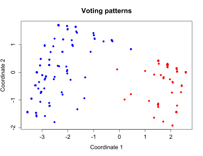
- Mapping the results and defining the dimensions – The statistical program (or a related module) will map the results. The map will plot each product (usually in two-dimensional space). The proximity of products to each other indicate either how similar they are or how preferred they are, depending on which approach was used. How the dimensions of the embedding actually correspond to dimensions of system behavior, however, are not necessarily obvious. Here, a subjective judgment about the correspondence can be made (see perceptual mapping).
- Test the results for reliability and validity – Compute R-squared to determine what proportion of variance of the scaled data can be accounted for by the MDS procedure. An R-square of 0.6 is considered the minimum acceptable level. An R-square of 0.8 is considered good for metric scaling and .9 is considered good for non-metric scaling. Other possible tests are Kruskal’s Stress, split data tests, data stability tests (i.e., eliminating one brand), and test-retest reliability.
- Report the results comprehensively – Along with the mapping, at least distance measure (e.g., Sorenson index, Jaccard index) and reliability (e.g., stress value) should be given. It is also very advisable to give the algorithm (e.g., Kruskal, Mather), which is often defined by the program used (sometimes replacing the algorithm report), if you have given a start configuration or had a random choice, the number of runs, the assessment of dimensionality, the Monte Carlo method results, the number of iterations, the assessment of stability, and the proportional variance of each axis (r-square).

Implementations
- ELKI includes two MDS implementations.
- Orange, a free data mining software suite, module orngMDS
- PC-ORD, Multivariate Analysis of Ecological Data command NMS
- MATLAB includes two MDS implementations (for classical (cmdscale) and non-classical (mdscale) MDS respectively).
- The R programming language offers several MDS implementations
- sklearn contains function sklearn.manifold.MDS
- usabiliTEST's Online Card Sorting software is utilizing MDS to plot the data collected from the participants of usability tests.
- ViSta has implementations of MDS by Forrest W. Young. Interactive graphics allow exploring the results of MDS in detail.
See also
| Wikimedia Commons has media related to Multidimensional scaling. |
- Positioning (marketing)
- Perceptual mapping
- Product management
- Marketing
- Generalized multidimensional scaling (GMDS)
- Data clustering
- Factor analysis
- Discriminant analysis
- Dimensionality reduction
- Nonlinear dimensionality reduction
- Distance geometry
- Cayley–Menger determinant
Bibliography
- 1 2 Borg, I., Groenen, P. (2005). Modern Multidimensional Scaling: theory and applications (2nd ed.). New York: Springer-Verlag. pp. 207–212. ISBN 0-387-94845-7.
- ↑ Wickelmaier, Florian. "An introduction to MDS." Sound Quality Research Unit, Aalborg University, Denmark (2003): 46
- ↑ Bronstein AM, Bronstein MM, Kimmel R (January 2006). "Generalized multidimensional scaling: a framework for isometry-invariant partial surface matching". Proc. Natl. Acad. Sci. U.S.A. 103 (5): 1168–72. doi:10.1073/pnas.0508601103. PMC 1360551
 . PMID 16432211.
 - ↑ Kruskal, J. B., and Wish, M. (1978), Multidimensional Scaling, Sage University Paper series on Quantitative Application in the Social Sciences, 07-011. Beverly Hills and London: Sage Publications.
- ↑ Kruskal, J. B. (1964). "Multidimensional scaling by optimizing goodness of fit to a nonmetric hypothesis". Psychometrika. 29 (1): 1–27. doi:10.1007/BF02289565.
- Cox, T.F., Cox, M.A.A. (2001). Multidimensional Scaling. Chapman and Hall.
- Coxon, Anthony P.M. (1982). The User's Guide to Multidimensional Scaling. With special reference to the MDS(X) library of Computer Programs. London: Heinemann Educational Books.
- Green, P. (January 1975). "Marketing applications of MDS: Assessment and outlook". Journal of Marketing. 39 (1): 24–31. doi:10.2307/1250799.
- McCune, B. & Grace, J.B. (2002). Analysis of Ecological Communities. Oregon, Gleneden Beach: MjM Software Design. ISBN 0-9721290-0-6.
- Torgerson, Warren S. (1958). Theory & Methods of Scaling. New York: Wiley. ISBN 0-89874-722-8.