Multidimensional transform
In mathematical analysis and applications, multidimensional transforms are used to analyze the frequency content of signals in a domain of two or more dimensions.
Multidimensional Fourier transform
One of the more popular multidimensional transforms is the Fourier transform, which converts a signal from a time/space domain representation to a frequency domain representation.[1] The discrete-domain multidimensional Fourier transform (FT) can be computed as follows:

where F stands for the multidimensional Fourier transform, m stands for multidimensional dimension. Define f as a multidimensional discrete-domain signal. The inverse multidimensional Fourier transform is given by

The multidimensional Fourier transform for continuous-domain signals is defined as follows:[1]

Properties of Fourier transform
Similar properties of the 1-D FT transform apply, but instead of the input parameter being just a single entry, it's a Multi-dimensional (MD) array or vector. Hence, it's x(n1,…,nM) instead of x(n).
Linearity
if , and then,


Shift
if , then


Modulation
if , then


Multiplication
if , and
then,
-
(MD Convolution in Frequency Domain)

or,
-
(MD Convolution in Frequency Domain)

Differentiation
If , then


Transposition
If , then

Reflection
If , then

Complex conjugation
If , then

Parseval's theorem (MD)
if , and then,


if , then


A special case of the Parseval's theorem is when the two multi-dimensional signals are the same. In this case, the theorem portrays the energy conservation of the signal and the term in the summation or integral is the energy-density of the signal.
Separability
One property is the separability property. A signal or system is said to be separable if it can be expressed as a product of 1-D functions with different independent variables. This phenomenon allows computing the FT transform as a product of 1-D FTs instead of multi-dimensional FT.
if , , ... , and if , then


, so


MD FFT
A fast Fourier transform (FFT) is an algorithm to compute the discrete Fourier transform (DFT) and its inverse. An FFT computes the DFT and produces exactly the same result as evaluating the DFT definition directly; the only difference is that an FFT is much faster. (In the presence of round-off error, many FFT algorithms are also much more accurate than evaluating the DFT definition directly).There are many different FFT algorithms involving a wide range of mathematics, from simple complex-number arithmetic to group theory and number theory. See more in FFT.
MD DFT
The multidimensional discrete Fourier transform (DFT) is a sampled version of the discrete-domain FT by evaluating it at sample frequencies that are uniformly spaced.[2] The N1 × N2 × ... NM DFT is given by:

for 0 ≤ Ki ≤ Ni − 1, i = 1, 2, ..., m.
The inverse multidimensional DFT equation is

for 0 ≤ n1, n2, ... , nm ≤ N(1, 2, ... , m) – 1.
Multidimensional discrete cosine transform
The discrete cosine transform (DCT) is used in a wide range of applications such as data compression, feature extraction, Image reconstruction, multi-frame detection and so on. The multidimensional DCT is given by:

for ki = 0, 1, ..., Ni − 1, i = 1, 2, ..., r.
Multidimensional Laplace transform
The multidimensional Laplace transform is useful for the solution of boundary value problems. Boundary value problems in two or more variables characterized by partial differential equations can be solved by a direct use of the Laplace transform.[3] The Laplace transform for an M-dimensional case is defined[3] as

where F stands for the s-domain representation of the signal f(t).
A special case (along 2 dimensions) of the multi-dimensional Laplace transform of function f(x,y) is defined[4] as

F(x,y) is called the image of f(x,y) and f(x,y) is known as the original of F(x,y).[5] This special case can be used to solve the Telegrapher's equations.[5]
Multidimensional Z transform[6]
The multidimensional Z transform is used to map the discrete time domain multidimensional signal to the Z domain. This can be used to check the stability of filters. The equation of the multidimensional Z transform is given by

where F stands for the z-domain representation of the signal f(n).
A special case of the multidimensional Z transform is the 2D Z transform which is given as

The Fourier transform is a special case of the Z transform evaluated along the unit circle (in 1D) and unit bi-circle (in 2D). i.e. at
where z and w are vectors.

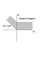
Region of convergence
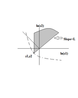
Points (z1,z2) for which are located in the ROC.


An example:
If a sequence has a support as shown in Figure 1.1a, then its ROC is shown in Figure 1.1b. This follows that |F(z1,z2)| < ∞ .
lies in the ROC, then all pointsthat satisfy |z1|≥|z01| and |z2|≥|z02 lie in the ROC.


Therefore, for figure 1.1a and 1.1b, the ROC would be

where L is the slope.
The 2D Z-transform, similar to the Z-transform, is used in multidimensional signal processing to relate a two-dimensional discrete-time signal to the complex frequency domain in which the 2D surface in 4D space that the Fourier transform lies on is known as the unit surface or unit bicircle.
Applications
The DCT and DFT are often used in signal processing[7] and image processing, and they are also used to efficiently solve partial differential equations by spectral methods. The DFT can also be used to perform other operations such as convolutions or multiplying large integers. The DFT and DCT have seen wide usage across a large number of fields, we only sketch a few examples below.
Image processing
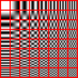
The DCT is used in JPEG image compression, MJPEG, MPEG, DV, Daala, and Theora video compression. There, the two-dimensional DCT-II of NxN blocks are computed and the results are quantized and entropy coded. In this case, N is typically 8 and the DCT-II formula is applied to each row and column of the block. The result is an 8x8 transform coefficient array in which the: (0,0) element (top-left) is the DC (zero-frequency) component and entries with increasing vertical and horizontal index values represent higher vertical and horizontal spatial frequencies, as shown in the picture on the right.
In image processing, one can also analyze and describe unconventional cryptographic methods based on 2D DCTs, for inserting non-visible binary watermarks into the 2D image plane,[8] and According to different orientations, the 2-D directional DCT-DWT hybrid transform can be applied in denoising ultrasound images.[9] 3-D DCT can also be used to transform video data or 3-D image data in watermark embedding schemes in transform domain.[10][11]
Spectral analysis
When the DFT is used for spectral analysis, the {xn} sequence usually represents a finite set of uniformly spaced time-samples of some signal x(t) where t represents time. The conversion from continuous time to samples (discrete-time) changes the underlying Fourier transform of x(t) into a discrete-time Fourier transform (DTFT), which generally entails a type of distortion called aliasing. Choice of an appropriate sample-rate (see Nyquist rate) is the key to minimizing that distortion. Similarly, the conversion from a very long (or infinite) sequence to a manageable size entails a type of distortion called leakage, which is manifested as a loss of detail (aka resolution) in the DTFT. Choice of an appropriate sub-sequence length is the primary key to minimizing that effect. When the available data (and time to process it) is more than the amount needed to attain the desired frequency resolution, a standard technique is to perform multiple DFTs, for example to create a spectrogram. If the desired result is a power spectrum and noise or randomness is present in the data, averaging the magnitude components of the multiple DFTs is a useful procedure to reduce the variance of the spectrum (also called a periodogram in this context); two examples of such techniques are the Welch method and the Bartlett method; the general subject of estimating the power spectrum of a noisy signal is called spectral estimation.
A final source of distortion (or perhaps illusion) is the DFT itself, because it is just a discrete sampling of the DTFT, which is a function of a continuous frequency domain. That can be mitigated by increasing the resolution of the DFT. That procedure is illustrated at Sampling the DTFT.
- The procedure is sometimes referred to as zero-padding, which is a particular implementation used in conjunction with the fast Fourier transform (FFT) algorithm. The inefficiency of performing multiplications and additions with zero-valued "samples" is more than offset by the inherent efficiency of the FFT.
- As already noted, leakage imposes a limit on the inherent resolution of the DTFT. So there is a practical limit to the benefit that can be obtained from a fine-grained DFT.
Partial differential equations
Discrete Fourier transforms are often used to solve partial differential equations, where again the DFT is used as an approximation for the Fourier series (which is recovered in the limit of infinite N). The advantage of this approach is that it expands the signal in complex exponentials einx, which are eigenfunctions of differentiation: d/dx einx = in einx. Thus, in the Fourier representation, differentiation is simple—we just multiply by i n. (Note, however, that the choice of n is not unique due to aliasing; for the method to be convergent, a choice similar to that in the trigonometric interpolation section above should be used.) A linear differential equation with constant coefficients is transformed into an easily solvable algebraic equation. One then uses the inverse DFT to transform the result back into the ordinary spatial representation. Such an approach is called a spectral method.
DCTs are also widely employed in solving partial differential equations by spectral methods, where the different variants of the DCT correspond to slightly different even/odd boundary conditions at the two ends of the array.
Laplace transforms are used to solve partial differential equations. The general theory for obtaining solutions in this technique is developed by theorems on Laplace transform in n dimensions.[3]
The multidimensional Z transform can also be used to solve partial differential equations.[12]
Image processing for arts surface analysis by FFT
One very important factor is that we must apply a non-destructive method to obtain those rare valuables information (from the HVS viewing point, is focused in whole colorimetric and spatial information) about works of art and zero-damage on them. We can understand the arts by looking at a color change or by measuring the surface uniformity change. Since the whole image will be very huge, so we use a double raised cosine window to truncate the image:[13]

where N is the image dimension and x, y are the coordinates from the center of image spans from 0 to N/2. The author wanted to compute an equal value for spatial frequency such as:[13]
![{\displaystyle {\begin{aligned}A_{m}(f)^{2}=\left[\sum _{i=-f}^{f}\right.&\operatorname {FFT} (-f,i)^{2}+\sum _{i=-f}^{f}\operatorname {FFT} (f,i)^{2}\\[5pt]&\left.{}+\sum _{i=-f+1}^{f-1}\operatorname {FFT} (i,-f)^{2}+\sum _{i=-f+1}^{f-1}\operatorname {FFT} (i,f)^{2}\right]\end{aligned}}}](../I/m/65e2b7dace8996c89cce35132a4f1e451800a219.svg)
where "FFT" denotes the fast Fourier transform, and f is the spatial frequency spans from 0 to N/2 – 1. The proposed FFT-based imaging approach is diagnostic technology to ensure a long life and stable to culture arts. This is a simple, cheap which can be used in museums without affecting their daily use. But this method doesn’t allow a quantitative measure of the corrosion rate.
Application to weakly nonlinear circuit simulation[14]
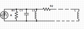
The inverse multidimensional Laplace transform can be applied to simulate nonlinear circuits. This is done so by formulating a circuit as a state-space and expanding the Inverse Laplace Transform based on Laguerre function expansion.
The Lagurre method can be used to simulate a weakly nonlinear circuit and the Laguerre method can invert a multidimensional Laplace transform efficiently with a high accuracy.
It is observed that a high accuracy and significant speedup can be achieved for simulating large nonlinear circuits using multidimensional Laplace transforms.
See also
- Discrete cosine transform
- List of Fourier-related transforms
- List of Fourier analysis topics
- Multidimensional discrete convolution
- 2D Z-transform
- Multidimensional empirical mode decomposition
- Multidimensional signal reconstruction
References
- 1 2 Smith,W. Handbook of Real-Time Fast Fourier Transforms:Algorithms to Product Testing, Wiley_IEEE Press, edition 1, pages 73–80, 1995
- ↑ Dudgeon and Mersereau, Multidimensional Digital Signal Processing,2nd edition,1995
- 1 2 3 Debnath, Joyati; Dahiya, R. S. (1989-01-01). "Theorems on multidimensional laplace transform for solution of boundary value problems". Computers & Mathematics with Applications. 18 (12): 1033–1056. doi:10.1016/0898-1221(89)90031-X.
- ↑ Operational Calculus in two Variables and its Application (1st English edition) - translated by D.M.G. Wishart (Calcul opérationnel).
- 1 2 Aghili and Moghaddam (2006). "Multi-Dimensional Laplace Transforms and Systems of Partial Differential Equations". International Mathematical Forum. 1 (21): 1043–1050.
- ↑ "Narod Book" (PDF).
- ↑ Tan Xiao, Shao-hai Hu, Yang Xiao. 2-D DFT-DWT Application to Multidimensional Signal Processing. ICSP2006 Proceedings, 2006 IEEE
- ↑ Peter KULLAI, Pavol SABAKAI, JozefHUSKAI. Simple Possibilities of 2D DCT Application in Digital Monochrome Image Cryptography. Radioelektronika, 17th International Conference, IEEE, 2007, pp. 1–6
- ↑ Xin-ling Wen, Yang Xiao. The 2-D Directional DCT-DWT Hybrid Transform and Its Application in Denoising Ultrasound Image. Signal Processing. ICSP 2008. 9th International Conference, Page(s): 946–949
- ↑ Jinwei Wang, Shiguo Lian, Zhongxuan Liu, Zhen Ren, Yuewei Dai, Haila Wang. Image Watermarking Scheme Based on 3-D DCT.Industrial Electronics and Applications, 2006 1ST IEEE Conference, pp. 1–6
- ↑ Jin Li, Moncef Gabbouj, Jarmo Takala, Hexin Chen. Direct 3-D DCT-to-DCT Resizing Algorithm for Video Coding. Image and Signal Processing and Analysis, 2009. ISPA 2009. Proceedings of 6th International Symposium pp. 105–110
- ↑ Gregor, Jiří (1998). "Kybernetika" (PDF). Kybernetika. 24.
- 1 2 Angelini, E., Grassin, S. ; Piantanida, M. ; Corbellini, S. ; Ferraris, F. ; Neri, A. ; Parvis, M. FFT-based imaging processing for cultural heritage monitoring Instrumentation and Measurement Technology Conference (I2MTC), 2010 IEEE
- ↑ Wang, Tingting (2012). "Weakly Nonlinear Circuit Analysis Based on Fast Multidimensional Inverse Laplace Transform". IEEE Conference Publications. doi:10.1109/ASPDAC.2012.6165013.