Radon transform

Radon transform. Maps f on the (x, y)-domain into f on the (α, s)-domain.

Radon transform of the indicator function of two squares shown in the image below. Lighter regions indicate larger function values. Black indicates zero.

Original function is equal to one on the white region and zero on the dark region.

In mathematics, the Radon transform is the integral transform which takes a function f defined on the plane to a function Rf defined on the (two-dimensional) space of lines in the plane, whose value at a particular line is equal to the line integral of the function over that line. The transform was introduced in 1917 by Johann Radon,^[1] who also provided a formula for the inverse transform. Radon further included formulas for the transform in three dimensions, in which the integral is taken over planes. It was later generalized to higher-dimensional Euclidean spaces, and more broadly in the context of integral geometry. The complex analog of the Radon transform is known as the Penrose transform.The Radon transform is widely applicable to tomography, the creation of an image from the projection data associated with cross-sectional scans of an object.

Shepp Logan phantom

Radon transform

Inverse Radon transform

Explanation

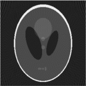
If a function $f$ represents an unknown density, then the Radon transform represents the projection data obtained as the output of a tomographic scan. Hence the inverse of the Radon transform can be used to reconstruct the original density from the projection data, and thus it forms the mathematical underpinning for tomographic reconstruction, also known as image reconstruction.

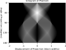
The Radon transform data is often called a sinogram because the Radon transform of an off-center point source is a sinusoid. Consequently the Radon transform of a number of small objects appears graphically as a number of blurred sine waves with different amplitudes and phases.

The Radon transform is useful in computed axial tomography (CAT scan), barcode scanners, electron microscopy of macromolecular assemblies like viruses and protein complexes, reflection seismology and in the solution of hyperbolic partial differential equations.

Definition

The (n-dimensional) Radon transform ${\mathcal {R}}$ maps a function on $\mathbb {R} ^{n}$ into the set of its integrals over the hyperplanes of $\mathbb {R} ^{n}$. More specifically, if ${\displaystyle \theta \in S^{n-1}}$ and ${\displaystyle s\in \mathbb {R} ^{1}}$,then

${\displaystyle {\mathcal {R}}f(\theta ,s)=\int \limits _{x\cdot \theta =s}f(x)dx=\int \limits _{\theta ^{\perp }}f(s\theta +y)dy}$

is the integral of $f$ over the hyperplane perpendicular to $\theta$ with (signed) distance $s$ from the origin.^[2]

In the 2D case, the Radon transform can be expressed as

${\displaystyle {\mathcal {R}}f(L)=\int _{L}f(\mathbf {x} )\,|d\mathbf {x} |.}$

Concretely, the parametrization of any straight line L with respect to arc length z can always be written

$(x(z),y(z))={\Big (}(z\sin \alpha +s\cos \alpha ),(-z\cos \alpha +s\sin \alpha ){\Big )}\,$

where s is the distance of L from the origin and $\alpha$ is the angle the normal vector to L makes with the x axis. It follows that the quantities (α,s) can be considered as coordinates on the space of all lines in R², and the Radon transform can be expressed in these coordinates by

${\displaystyle {\begin{aligned}{\mathcal {R}}f(\alpha ,s)&=\int _{-\infty }^{\infty }f(x(z),y(z))\,dz\\&=\int _{-\infty }^{\infty }f{\big (}(z\sin \alpha +s\cos \alpha ),(-z\cos \alpha +s\sin \alpha ){\big )}\,dz\end{aligned}}}$

Relationship with the Fourier transform

The Radon transform is closely related to the Fourier transform. For a function of one variable the Fourier transform is defined by

${\hat {f}}(\omega )=\int _{-\infty }^{\infty }f(x)e^{-2\pi ix\omega }\,dx.$

and for a function of a 2-vector $\mathbf {x} =(x,y)$,

${\hat {f}}(\mathbf {w} )=\int \limits _{-\infty }^{\infty }\int \limits _{-\infty }^{\infty }f(\mathbf {x} )e^{-2\pi i\mathbf {x} \cdot \mathbf {w} }\,dx\,dy.$

For convenience, denote ${\displaystyle {\mathcal {R}}_{\alpha }[f](s)={\mathcal {R}}[f](\alpha ,s)}$. The Fourier slice theorem then states

${\displaystyle {\widehat {{\mathcal {R}}_{\alpha }[f]}}(\sigma )={\hat {f}}(\sigma \mathbf {n} (\alpha ))}$

where

$\mathbf {n} (\alpha )=(\cos \alpha ,\sin \alpha ).$

Thus the two-dimensional Fourier transform of the initial function along a line at the inclination angle $\alpha$ is the one variable Fourier transform of the Radon transform (acquired at angle $\alpha$) of that function.

More generally, one has the result valid in n dimensions

${\displaystyle {\hat {f}}(r\alpha )=\int _{-\infty }^{\infty }{\mathcal {R}}f(\alpha ,s)e^{-2\pi isr}\,ds.}$

Dual transform

The dual Radon transform is a kind of adjoint to the Radon transform. Beginning with a function g on the space Σ_n, the dual Radon transform is the function ${\displaystyle {\mathcal {R}}^{*}g}$ on Rⁿ defined by

${\displaystyle {\mathcal {R}}^{*}g(x)=\int _{x\in \xi }g(\xi )\,d\mu (\xi ).}$

The integral here is taken over the set of all lines incident with the point x ∈ Rⁿ, and the measure dμ is the unique probability measure on the set $\{\xi |x\in \xi \}$ invariant under rotations about the point x.

Concretely, for the two-dimensional Radon transform, the dual transform is given by

${\displaystyle {\mathcal {R}}^{*}g(x)={\frac {1}{2\pi }}\int _{\alpha =0}^{2\pi }g(\alpha ,\mathbf {n} (\alpha )\cdot \mathbf {x} )\,d\alpha .}$

In the context of image processing, the dual transform is commonly called backprojection^[3] as it takes a function defined on each line in the plane and 'smears' or projects it back over the line to produce an image.

Intertwining property

Let Δ denote the Laplacian on Rⁿ:

$\Delta ={\frac {\partial ^{2}}{\partial x_{1}^{2}}}+\cdots +{\frac {\partial ^{2}}{\partial x_{n}^{2}}}.$

This is a natural rotationally invariant second-order differential operator. On Σ_n, the "radial" second derivative

$Lf(\alpha ,s)\equiv {\frac {\partial ^{2}}{\partial s^{2}}}f(\alpha ,s)$

is also rotationally invariant. The Radon transform and its dual are intertwining operators for these two differential operators in the sense that^[4]

${\displaystyle {\mathcal {R}}(\Delta f)=L({\mathcal {R}}f),\quad {\mathcal {R}}^{*}(Lg)=\Delta ({\mathcal {R}}^{*}g).}$

Reconstruction approaches

The process of reconstruction produces the image (or function $f$ in the previous section) from its projection data. Reconstruction is an inverse problem.

Radon inversion formula

In the 2D case, the most commonly used analytical formula to recover $f$ from its Radon transform is the Filtered Backprojection Formula or Radon Inversion Formula:

${\displaystyle f(\mathbf {x} )=\int _{0}^{\pi }({\mathcal {R}}f(\cdot ,\theta )*h)(<\mathbf {x} ,\mathbf {n} _{\theta }>)d\theta }$^[5]

where $h$ is such that ${\displaystyle {\hat {h}}(k)=|k|}$. ^[6]

The convolution kernel $h$ is referred to as Ramp filter in some literature.

Ill-posedness

Intuitively, in the filtered backprojection formula, by analogy with differentiation, for which ${\displaystyle {\widehat {\frac {d}{dx}}}f(k)=ik{\widehat {f}}(k)}$, we see that the filter performs an operation similar to a derivative. Roughly speaking, then, the filter makes objects more singular.

A quantitive statement of the ill-posedness of Radon Inversion goes as follows:

We have ${\displaystyle {\widehat {{\mathcal {R}}^{*}{\mathcal {R}}g}}(k)={\frac {1}{||\mathbf {k} ||}}{\hat {g}}(\mathbf {k} )}$

where ${\displaystyle {\mathcal {R}}^{*}}$ is the previously defined adjoint to the Radon Transform.

Thus for ${\displaystyle g(\mathbf {x} )=e^{i<\mathbf {k} _{0},\mathbf {x} >}}$,

${\displaystyle {\mathcal {R}}^{*}{\mathcal {R}}g={\frac {1}{||\mathbf {k_{0}} ||}}e^{i<\mathbf {k} _{0},\mathbf {x} >}}$.

The complex exponential ${\displaystyle e^{i<\mathbf {k} _{0},\mathbf {x} >}}$ is thus an eigenfunction of ${\displaystyle {\mathcal {R}}^{*}{\mathcal {R}}}$ with eigenvalue ${\displaystyle {\frac {1}{||\mathbf {k_{0}} ||}}}$. Thus the singular values of ${\mathcal {R}}$ are ${\displaystyle {\sqrt {\frac {1}{||\mathbf {k} ||}}}}$. Since these singular values tend to 0, ${\displaystyle {\mathcal {R}}^{-1}}$ is unbounded. ^[6]

Iterative Reconstruction methods

Compared with the Filtered Backprojection method, iterative reconstruction costs large computation time, limiting its pratical use. However, due to the ill-posedness of Radon Inversion, the Filtered Backprojection method may be infeasible in the presence of discontinuity or noise. The iterative reconstruction could provide metal artifact reduction, noise and dose reduction for the reconstructed result that attract much research interest around the world. ^[7]

See also

• Deconvolution
• X-ray transform
• Funk transform
• The Hough transform, when written in a continuous form, is very similar, if not equivalent, to the Radon transform.^[8]
• Cauchy-Crofton theorem is a closely related formula for computing the length of curves in space.
• Fourier transform

Notes

1. Radon 1917.
2. Natterer, F. (1986). The Mathematics of Computerized Tomography. p. 9. ISBN 0 471 90959 9.
3. Roerdink 2001
4. Helgason 1984, Lemma I.2.1
5. Candès, Emmanuel. "Applied Fourier Analysis and Elements of Modern Signal Processing - Lecture 9" (PDF).
6. Candès, Emmanuel. "Applied Fourier Analysis and Elements of Modern Signal Processing - Lecture 10" (PDF).
7. Lalush, David. "Iterative reconstruction methods and applications" (PDF).
8. van Ginkel, M.; Luengo Hendricks, C.L.; van Vliet, L.J. "A short introduction to the Radon and Hough transforms and how they relate to each other" (PDF). Archived (PDF) from the original on 2016-07-29.

References

• Deans, Stanley R. (1983), The Radon Transform and Some of Its Applications, New York: John Wiley & Sons.
• Helgason, Sigurdur (2008), Geometric analysis on symmetric spaces, Mathematical Surveys and Monographs, 39 (2nd ed.), Providence, R.I.: American Mathematical Society, ISBN 978-0-8218-4530-1, MR 2463854.
• Helgason, Sigurdur (1984), Groups and Geometric Analysis: Integral Geometry, Invariant Differential Operators, and Spherical Functions, Academic Press, ISBN 0-12-338301-3.
• Herman, Gabor T. (2009), Fundamentals of Computerized Tomography: Image Reconstruction from Projections (2nd ed.), Springer, ISBN 978-1-85233-617-2.
• Minlos, R.A. (2001), "Radon transform", in Hazewinkel, Michiel, Encyclopedia of Mathematics, Springer, ISBN 978-1-55608-010-4.
• Natterer, Frank, The Mathematics of Computerized Tomography, Classics in Applied Mathematics, 32, Society for Industrial and Applied Mathematics, ISBN 0-89871-493-1
• Natterer, Frank; Wübbeling, Frank, Mathematical Methods in Image Reconstruction, Society for Industrial and Applied Mathematics, ISBN 0-89871-472-9.
• Radon, Johann (1917), "Über die Bestimmung von Funktionen durch ihre Integralwerte längs gewisser Mannigfaltigkeiten", Berichte über die Verhandlungen der Königlich-Sächsischen Akademie der Wissenschaften zu Leipzig, Mathematisch-Physische Klasse [Reports on the proceedings of the Royal Saxonian Academy of Sciences at Leipzig, mathematical and physical section], Leipzig: Teubner (69): 262–277; Translation: Radon, J.; Parks, P.C. (translator) (1986), "On the determination of functions from their integral values along certain manifolds", IEEE Transactions on Medical Imaging, 5 (4): 170–176, doi:10.1109/TMI.1986.4307775, PMID 18244009.
• Roerdink, J.B.T.M. (2001), "Tomography", in Hazewinkel, Michiel, Encyclopedia of Mathematics, Springer, ISBN 978-1-55608-010-4.
• Weisstein, Eric W. "Radon transform". MathWorld.

.