Riemann sum

Four of the Riemann summation methods for approximating the area under curves. Right and left methods make the approximation using the right and left endpoints of each subinterval, respectively. Maximum and minimum methods make the approximation using the largest and smallest endpoint values of each subinterval, respectively. The values of the sums converge as the subintervals halve from top-left to bottom-right.

In mathematics, a Riemann sum is an approximation that takes the form $\sum f(x)\Delta x$. It is named after German mathematician Bernhard Riemann. One very common application is approximating the area of functions or lines on a graph, but also the length of curves and other approximations.

The sum is calculated by dividing the region up into shapes (rectangles, trapezoids, parabolas, or cubics) that together form a region that is similar to the region being measured, then calculating the area for each of these shapes, and finally adding all of these small areas together. This approach can be used to find a numerical approximation for a definite integral even if the fundamental theorem of calculus does not make it easy to find a closed-form solution.

Because the region filled by the small shapes is usually not exactly the same shape as the region being measured, the Riemann sum will differ from the area being measured. This error can be reduced by dividing up the region more finely, using smaller and smaller shapes. As the shapes get smaller and smaller, the sum approaches the Riemann integral.

Definition

Let f : D → R be a function defined on a subset, D, of the real line, R. Let I = [a, b] be a closed interval contained in D, and let

$P=\left\{[x_{0},x_{1}],[x_{1},x_{2}],\dots ,[x_{n-1},x_{n}]\right\},$

be a partition of I, where

$a=x_{0}<x_{1}<x_{2}<\cdots <x_{n}=b.$

A Riemann sum of f over I with partition P is defined as

$S=\sum _{i=1}^{n}f(x_{i}^{*})(x_{i}-x_{i-1}),\quad x_{i-1}\leq x_{i}^{*}\leq x_{i}.$

Notice the use of "a" instead of "the" in the previous sentence. This is due to the fact that the choice of $x_{i}^{*}$ in the interval $[x_{i-1},x_{i}]$ is arbitrary, so for any given function f defined on an interval I and a fixed partition P, one might produce different Riemann sums depending on which $x_{i}^{*}$ is chosen, as long as $x_{i-1}\leq x_{i}^{*}\leq x_{i}$ holds true.

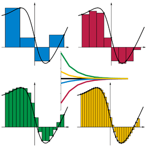
Example: Specific choices of $x_{i}^{*}$ give us different types of Riemann sums:

• If $x_{i}^{*}=x_{i-1}$ for all i, then S is called a left Riemann sum.
• If $x_{i}^{*}=x_{i}$ for all i, then S is called a right Riemann sum.
• If $x_{i}^{*}={\tfrac {1}{2}}(x_{i}+x_{i-1})$ for all i, then S is called a middle Riemann sum.
• The average of the left and right Riemann sum is the trapezoidal sum.
• If it is given that

$S=\sum _{i=1}^{n}v_{i}(x_{i}-x_{i-1}),$

where $v_{i}$ is the supremum of f over $[x_{i-1},x_{i}]$, then S is defined to be an upper Riemann sum.

• Similarly, if $v_{i}$ is the infimum of f over $[x_{i-1},x_{i}]$, then S is a lower Riemann sum.

Riemann sum methods of x³ over [0,2] using 4 subdivisions

Left

Right

Middle

Trapezoidal

Simpson's Method

Any Riemann sum on a given partition (that is, for any choice of $x_{i}^{*}$ between $x_{i-1}$ and $x_{i}$) is contained between the lower and the upper Riemann sums. A function is defined to be Riemann integrable if the lower and upper Riemann sums get ever closer as the partition gets finer and finer. This fact can also be used for numerical integration.

Methods

The four methods of Riemann summation are usually best approached with partitions of equal size. The interval [a, b] is therefore divided into n subintervals, each of length

$\Delta x={\frac {b-a}{n}}.$

The points in the partition will then be

$a,a+\Delta x,a+2\Delta x,\ldots ,a+(n-2)\Delta x,a+(n-1)\Delta x,b.$

Left Riemann Sum

For the left Riemann sum, approximating the function by its value at the left-end point gives multiple rectangles with base Δx and height f(a + iΔx). Doing this for i = 0, 1, ..., n − 1, and adding up the resulting areas gives

$\Delta x\left[f(a)+f(a+\Delta x)+f(a+2\Delta x)+\cdots +f(b-\Delta x)\right].$

The left Riemann sum amounts to an overestimation if f is monotonically decreasing on this interval, and an underestimation if it is monotonically increasing.

Right Riemann Sum

f is here approximated by the value at the right endpoint. This gives multiple rectangles with base Δx and height f(a + iΔx). Doing this for i = 1, ..., n, and adding up the resulting areas produces

$\Delta x \left[ f( a + \Delta x ) + f(a + 2 \Delta x)+\cdots+f(b) \right].$

The right Riemann sum amounts to an underestimation if f is monotonically decreasing, and an overestimation if it is monotonically increasing. The error of this formula will be

$\left \vert \int_{a}^{b} f(x) \, dx - A_\mathrm{right} \right \vert \le \frac{M_1 (b-a)^2}{2n},$

where $M_{1}$ is the maximum value of the absolute value of $f^{\prime}(x)$ on the interval.

Middle sum

Approximating f at the midpoint of intervals gives f(a + Δx/2) for the first interval, for the next one f(a + 3Δx/2), and so on until f(b − Δx/2). Summing up the areas gives

$\Delta x\left[f(a+{\tfrac {\Delta x}{2}})+f(a+{\tfrac {3\Delta x}{2}})+\cdots +f(b-{\tfrac {\Delta x}{2}})\right].$

The error of this formula will be

$\left\vert \int _{a}^{b}f(x)\,dx-A_{\mathrm {mid} }\right\vert \leq {\frac {M_{2}(b-a)^{3}}{24n^{2}}},$

where $M_{2}$ is the maximum value of the absolute value of $f^{\prime \prime }(x)$ on the interval.

Trapezoidal Rule

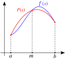
In this case, the values of the function f on an interval are approximated by the average of the values at the left and right endpoints. In the same manner as above, a simple calculation using the area formula

$A={\tfrac {1}{2}}h(b_{1}+b_{2})$

for a trapezium with parallel sides b₁, b₂ and height h produces

${\tfrac {1}{2}}\Delta x\left[f(a)+2f(a+\Delta x)+2f(a+2\Delta x)+2f(a+3\Delta x)+\cdots +f(b)\right].$

The error of this formula will be

$\left\vert \int _{a}^{b}f(x)\,dx-A_{\mathrm {trap} }\right\vert \leq {\frac {M_{2}(b-a)^{3}}{12n^{2}}},$

where $M_{2}$ is the maximum value of the absolute value of $f^{\prime \prime }(x).$

The approximation obtained with the trapezoid rule for a function is the same as the average of the left hand and right hand sums of that function.

Example

A visual representation of the area under the curve y = x² for the interval from 0 to 2

The value of the Riemann sum under the curve y = x² from 0 to 2. As the number of rectangles increases, it approaches the exact area of 8/3.

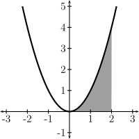
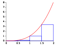
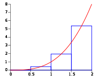
Taking an example, the area under the curve of y = x² between 0 and 2 can be procedurally computed using Riemann's method.

The interval [0, 2] is firstly divided into n subintervals, each of which is given a width of ${\tfrac {2}{n}}$; these are the widths of the Riemann rectangles (hereafter "boxes"). Because the right Riemann sum is to be used, the sequence of x coordinates for the boxes will be $x_{1},x_{2},\ldots ,x_{n}$. Therefore, the sequence of the heights of the boxes will be $x_{1}^{2},x_{2}^{2},\ldots ,x_{n}^{2}$. It is an important fact that $x_{i}={\tfrac {2i}{n}}$, and $x_{n}=2$.

The area of each box will be ${\tfrac {2}{n}}\times x_{i}^{2}$ and therefore the nth right Riemann sum will be:

${\begin{aligned}S&={\frac {2}{n}}\times \left({\frac {2}{n}}\right)^{2}+\cdots +{\frac {2}{n}}\times \left({\frac {2i}{n}}\right)^{2}+\cdots +{\frac {2}{n}}\times \left({\frac {2n}{n}}\right)^{2}\\&={\frac {8}{n^{3}}}\left(1+\cdots +i^{2}+\cdots +n^{2}\right)\\&={\frac {8}{n^{3}}}\left({\frac {n(n+1)(2n+1)}{6}}\right)\\&={\frac {8}{n^{3}}}\left({\frac {2n^{3}+3n^{2}+n}{6}}\right)\\&={\frac {8}{3}}+{\frac {4}{n}}+{\frac {4}{3n^{2}}}\end{aligned}}$

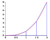
If the limit is viewed as n → ∞, it can be concluded that the approximation approaches the actual value of the area under the curve as the number of boxes increases. Hence:

$\lim _{n\to \infty }S=\lim _{n\to \infty }\left({\frac {8}{3}}+{\frac {4}{n}}+{\frac {4}{3n^{2}}}\right)={\frac {8}{3}}$

This method agrees with the definite integral as calculated in more mechanical ways:

$\int _{0}^{2}x^{2}\,dx={\frac {8}{3}}$

Animations

• 

  Left sum

• 

  Right sum

• 

  Middle sum

• 

  With $y=x^{2}$

See also

• Riemann integral
• Riemann–Stieltjes integral
• Lebesgue integral
• Simpson's rule
• Euler method and midpoint method, related methods for solving differential equations
• Antiderivative

References

• Thomas, George B. Jr.; Finney, Ross L. (1996), Calculus and Analytic Geometry (9th ed.), Addison Wesley, ISBN 0-201-53174-7

External links

• A simulation showing the convergence of Riemann sums