Riemann integral

The integral as the area of a region under a curve.

A sequence of Riemann sums over a regular partition of an interval. The number on top is the total area of the rectangles, which converges to the integral of the function.

The partition does not need to be regular, as shown here. The approximation works as long as the width of each subdivision tends to zero.

In the branch of mathematics known as real analysis, the Riemann integral, created by Bernhard Riemann, was the first rigorous definition of the integral of a function on an interval.^[1] For many functions and practical applications, the Riemann integral can be evaluated by the fundamental theorem of calculus or approximated by numerical integration.

The Riemann integral is unsuitable for many theoretical purposes. Some of the technical deficiencies in Riemann integration can be remedied with the Riemann–Stieltjes integral, and most disappear with the Lebesgue integral.

Overview

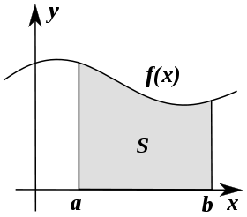
Let f be a non-negative real-valued function on the interval [a, b] , and let

$S = \left \{ (x, y) \, : \ a \leq x \leq b, 0 < y < f(x) \right \}$

be the region of the plane under the graph of the function f and above the interval [a, b] (see the figure on the top right). We are interested in measuring the area of S . Once we have measured it, we will denote the area by:

$\int_{a}^{b}f(x)\,dx.$

The basic idea of the Riemann integral is to use very simple approximations for the area of S . By taking better and better approximations, we can say that "in the limit" we get exactly the area of S under the curve.

Note that where f can be both positive and negative, the definition of S is modified so that the integral corresponds to the signed area under the graph of f : that is, the area above the x -axis minus the area below the x -axis.

Definition

Partitions of an interval

A partition of an interval $[a,b]$ is a finite sequence of numbers of the form

${\displaystyle a=x_{0}<x_{1}<x_{2}<\dots <x_{n}=b}$

Each $[x_i, x_{i+1}]$ is called a subinterval of the partition. The mesh or norm of a partition is defined to be the length of the longest subinterval, that is,

$\max (x_{i+1}-x_i), \quad i \in [0,n-1].$

A tagged partition $P(x,t)$ of an interval $[a,b]$ is a partition together with a finite sequence of numbers $t_0,\dots,t_{n-1}$ subject to the conditions that for each $i$, $t_i \in [x_i,x_{i+1}]$. In other words, it is a partition together with a distinguished point of every subinterval. The mesh of a tagged partition is the same as that of an ordinary partition.

Suppose that two partitions $P(x,t)$ and $Q(y,s)$ are both partitions of the interval $[a,b]$. We say that $Q(y,s)$ is a refinement of $P(x,t)$ if for each integer $i$, with $i \in [0,n]$, there exists an integer $r(i)$ such that $x_i=y_{r(i)}$ and such that $t_i=s_j$ for some $j$ with $j \in [r(i),r(i+1))$. Said more simply, a refinement of a tagged partition breaks up some of the subintervals and adds tags to the partition where necessary, thus it "refines" the accuracy of the partition.

We can define a partial order on the set of all tagged partitions by saying that one tagged partition is greater or equal to another if the former is a refinement of the latter.

Riemann sums

Choose a real-valued function $f$ which is defined on the interval $[a,b]$. The Riemann sum of $f$ with respect to the tagged partition $x_{0},\dots ,x_{n}$ together with $t_0,\dots,t_{n-1}$ is^[2]

$\sum_{i=0}^{n-1} f(t_i) (x_{i+1}-x_i).$

Each term in the sum is the product of the value of the function at a given point, and the length of an interval. Consequently, each term represents the (signed) area of a rectangle with height $f(t_i)$ and width $x_{i+1}-x_i$. The Riemann sum is the (signed) area of all the rectangles.

A closely related concept are the lower and upper Darboux sums. These are similar to Riemann sums, but the tags are replaced by the infimum and supremum (respectively) of f on each subinterval:

${\displaystyle L(f,P)=\sum _{i=0}^{n-1}\inf _{t\in [x_{i},x_{i+1}]}f(t)(x_{i+1}-x_{i}),}$

${\displaystyle U(f,P)=\sum _{i=0}^{n-1}\sup _{t\in [x_{i},x_{i+1}]}f(t)(x_{i+1}-x_{i}).}$

If f is continuous, then the lower and upper Darboux sums for an untagged partition are equal to the Riemann sum for that partition, where the tags are chosen to be the minimum or maximum (respectively) of f on each subinterval. (When f is discontinuous on a subinterval, there may not be a tag that achieves the infimum or supremum on that subinterval.) The Darboux integral, which is similar to the Riemann integral but based on Darboux sums, is equivalent to the Riemann integral.

Riemann integral

Loosely speaking, the Riemann integral is the limit of the Riemann sums of a function as the partitions get finer. If the limit exists then the function is said to be integrable (or more specifically Riemann-integrable). The Riemann sum can be made as close as desired to the Riemann integral by making the partition fine enough.^[3]

One important requirement is that the mesh of the partitions must become smaller and smaller, so that in the limit, it is zero. If this were not so, then we would not be getting a good approximation to the function on certain subintervals. In fact, this is enough to define an integral. To be specific, we say that the Riemann integral of f equals s if the following condition holds:

For all ε > 0, there exists δ such that for any tagged partition $x_0,\ldots,x_n$ and $t_0,\ldots,t_{n-1}$ whose mesh is less than δ, we have

$\left|\sum_{i=0}^{n-1} f(t_i) (x_{i+1}-x_i) - s\right| < \varepsilon.$

Unfortunately, this definition is very difficult to use. It would help to develop an equivalent definition of the Riemann integral which is easier to work with. We develop this definition now, with a proof of equivalence following. Our new definition says that the Riemann integral of f equals s if the following condition holds:

For all ε > 0, there exists a tagged partition $y_0,\ldots,y_m$ and $r_0,\ldots,r_{m-1}$ such that for any tagged partition $x_0, \ldots, x_n$ and $t_0,\ldots,t_{n-1}$ which is a refinement of $y_0,\ldots,y_m$ and $r_0,\ldots,r_{m-1}$, we have

$\left|\sum_{i=0}^{n-1} f(t_i) (x_{i+1}-x_i) - s\right| < \varepsilon.$

Both of these mean that eventually, the Riemann sum of f with respect to any partition gets trapped close to s. Since this is true no matter how close we demand the sums be trapped, we say that the Riemann sums converge to s. These definitions are actually a special case of a more general concept, a net.

As we stated earlier, these two definitions are equivalent. In other words, s works in the first definition if and only if s works in the second definition. To show that the first definition implies the second, start with an ε, and choose a δ that satisfies the condition. Choose any tagged partition whose mesh is less than δ. Its Riemann sum is within ε of s, and any refinement of this partition will also have mesh less than δ, so the Riemann sum of the refinement will also be within ε of s.

To show that the second definition implies the first, it is easiest to use the Darboux integral. First, one shows that the second definition is equivalent to the definition of the Darboux integral; for this see the article on Darboux integration. Now we will show that a Darboux integrable function satisfies the first definition. Fix ε, and choose a partition $y_0, \ldots, y_m$ such that the lower and upper Darboux sums with respect to this partition are within $\tfrac{\varepsilon}{2}$ of the value s of the Darboux integral. Let

${\displaystyle r=2\sup _{x\in [a,b]}|f(x)|.}$

If r = 0, then f is the zero function, which is clearly both Darboux and Riemann integrable with integral zero. Therefore, we will assume that r > 0. If m > 1, then we choose δ such that

$\delta < \min \left \{\frac{\varepsilon}{2r(m-1)}, (y_1 - y_0), (y_2 - y_1), \cdots, (y_m - y_{m-1}) \right \}$

If m = 1, then we choose δ to be less than one. Choose a tagged partition $x_0,\ldots,x_n$ and $t_0,\ldots,t_{n-1}$ with mesh smaller than δ. We must show that the Riemann sum is within ε of s .

To see this, choose an interval $[x_i,x_{i+1}]$. If this interval is contained within some $[y_j,y_{j+1}]$, then

$m_j < f(t_i) < M_j$

where m_j and M_j are respectively, the infimum and the supremum of f on $[y_j,y_{j+1}]$. If all intervals had this property, then this would conclude the proof, because each term in the Riemann sum would be bounded by a corresponding term in the Darboux sums, and we chose the Darboux sums to be near s. This is the case when m = 1, so the proof is finished in that case.

Therefore, we may assume that m > 1. In this case, it is possible that one of the $[x_i,x_{i+1}]$ is not contained in any $[y_j,y_{j+1}]$. Instead, it may stretch across two of the intervals determined by $y_0, \ldots, y_m$. (It cannot meet three intervals because δ is assumed to be smaller than the length of any one interval.) In symbols, it may happen that

$y_j < x_i < y_{j+1} < x_{i+1} < y_{j+2}.$

(We may assume that all the inequalities are strict because otherwise we are in the previous case by our assumption on the length of δ.) This can happen at most m−1 times.

To handle this case, we will estimate the difference between the Riemann sum and the Darboux sum by subdividing the partition $x_0,\ldots,x_n$ at $y_{j+1}$. The term $f(t_i)(x_{i+1}-x_i)$ in the Riemann sum splits into two terms:

$f(t_i)(x_{i+1}-x_i) = f(t_i)(x_{i+1}-y_{j+1})+f(t_i)(y_{j+1}-x_i).$

Suppose, without loss of generality, that $t_i \in [y_j,y_{j+1}]$. Then

$m_j < f(t_i) < M_j,$

so this term is bounded by the corresponding term in the Darboux sum for y_j. To bound the other term, notice that

$x_{i+1}-y_{j+1} < \delta < \frac{\varepsilon}{2r(m-1)},$

It follows that, for some (indeed any) ${\displaystyle t_{i}^{*}\in [y_{j+1},x_{i+1}]}$,

${\displaystyle |f(t_{i})-f(t_{i}^{*})|(x_{i+1}-y_{j+1})<{\frac {\varepsilon }{2(m-1)}}.}$

Since this happens at most m−1 times, the distance between the Riemann sum and a Darboux sum is at most $\tfrac{\varepsilon}{2}$. Therefore, the distance between the Riemann sum and s is at most ε.

Examples

Let $f:[0,1] \to \mathbf{R}$ be the function which takes the value 1 at every point. Any Riemann sum of f on [0, 1] will have the value 1, therefore the Riemann integral of f on [0, 1] is 1.

Let $I_{\mathbf{Q}}:[0,1] \to \mathbf{R}$ be the indicator function of the rational numbers in [0, 1]; that is, I_Q takes the value 1 on rational numbers and 0 on irrational numbers. This function does not have a Riemann integral. To prove this, we will show how to construct tagged partitions whose Riemann sums get arbitrarily close to both zero and one.

To start, let $x_0, \ldots, x_n$ and $t_0, \ldots, t_{n-1}$ be a tagged partition (each t_i is between x_i and $x_{i+1}$). Choose ε > 0. The t_i have already been chosen, and we can't change the value of f at those points. But if we cut the partition into tiny pieces around each t_i, we can minimize the effect of the t_i. Then, by carefully choosing the new tags, we can make the value of the Riemann sum turn out to be within ε of either zero or one—our choice!

Our first step is to cut up the partition. There are n of the t_i, and we want their total effect to be less than ε. If we confine each of them to an interval of length less than $\tfrac{\varepsilon}{n}$, then the contribution of each t_i to the Riemann sum will be at least $\tfrac{(0\cdot\varepsilon)}{n}$ and at most $\tfrac{(1\cdot\varepsilon)}{n}$. This makes the total sum at least zero and at most ε. So let δ be a positive number less than $\tfrac{\varepsilon}{n}$. If it happens that two of the t_i are within δ of each other, choose δ smaller. If it happens that some t_i is within δ of some x_j, and t_i is not equal to x_j, choose δ smaller. Since there are only finitely many t_i and x_j, we can always choose δ sufficiently small.

Now we add two cuts to the partition for each t_i. One of the cuts will be at $t_i - \tfrac{\delta}{2}$, and the other will be at $t_i + \tfrac{\delta}{2}$. If one of these leaves the interval [0, 1], then we leave it out. t_i will be the tag corresponding to the subinterval

$\left [t_i - \tfrac{\delta}{2}, t_i + \tfrac{\delta}{2} \right ].$

If t_i is directly on top of one of the x_j, then we let t_i be the tag for both intervals:

$\left [t_i - \tfrac{\delta}{2}, x_j \right ], \quad \left [x_j,t_i + \tfrac{\delta}{2} \right ].$

We still have to choose tags for the other subintervals. We will choose them in two different ways. The first way is to always choose a rational point, so that the Riemann sum is as large as possible. This will make the value of the Riemann sum at least 1−ε. The second way is to always choose an irrational point, so that the Riemann sum is as small as possible. This will make the value of the Riemann sum at most ε.

Since we started from an arbitrary partition and ended up as close as we wanted to either zero or one, it is false to say that we are eventually trapped near some number s, so this function is not Riemann integrable. However, it is Lebesgue integrable. In the Lebesgue sense its integral is zero, since the function is zero almost everywhere. But this is a fact that is beyond the reach of the Riemann integral.

There are even worse examples. I_Q is equivalent (that is, equal almost everywhere) to a Riemann integrable function, but there are non-Riemann integrable bounded functions which are not equivalent to any Riemann integrable function. For example, let C be the Smith–Volterra–Cantor set, and let I_C be its indicator function. Because C is not Jordan measurable, I_C is not Riemann integrable. Moreover, no function g equivalent to I_C is Riemann integrable: g, like I_C, must be zero on a dense set, so as in the previous example, any Riemann sum of g has a refinement which is within ε of 0 for any positive number ε. But if the Riemann integral of g exists, then it must equal the Lebesgue integral of I_C, which is 1/2. Therefore, g is not Riemann integrable.

Similar concepts

It is popular to define the Riemann integral as the Darboux integral. This is because the Darboux integral is technically simpler and because a function is Riemann-integrable if and only if it is Darboux-integrable.

Some calculus books do not use general tagged partitions, but limit themselves to specific types of tagged partitions. If the type of partition is limited too much, some non-integrable functions may appear to be integrable.

One popular restriction is the use of "left-hand" and "right-hand" Riemann sums. In a left-hand Riemann sum, $t_i = x_i$ for all i, and in a right-hand Riemann sum, $t_i = x_{i+1}$ for all i. Alone this restriction does not impose a problem: we can refine any partition in a way that makes it a left-hand or right-hand sum by subdividing it at each t_i. In more formal language, the set of all left-hand Riemann sums and the set of all right-hand Riemann sums is cofinal in the set of all tagged partitions.

Another popular restriction is the use of regular subdivisions of an interval. For example, the $n'$th regular subdivision of [0, 1] consists of the intervals

$\left [0, \tfrac{1}{n} \right], \left [\tfrac{1}{n}, \tfrac{2}{n} \right], \ldots, \left[\tfrac{n-1}{n}, 1 \right].$

Again, alone this restriction does not impose a problem, but the reasoning required to see this fact is more difficult than in the case of left-hand and right-hand Riemann sums.

However, combining these restrictions, so that one uses only left-hand or right-hand Riemann sums on regularly divided intervals, is dangerous. If a function is known in advance to be Riemann integrable, then this technique will give the correct value of the integral. But under these conditions the indicator function I_Q will appear to be integrable on [0, 1] with integral equal to one: Every endpoint of every subinterval will be a rational number, so the function will always be evaluated at rational numbers, and hence it will appear to always equal one. The problem with this definition becomes apparent when we try to split the integral into two pieces. The following equation ought to hold:

$\int_0^{\sqrt{2}-1}\! I_\mathbf{Q}(x) \,\mathrm{d}x + \int_{\sqrt{2}-1}^1\! I_\mathbf{Q}(x) \,\mathrm{d}x = \int_0^1\! I_\mathbf{Q}(x) \,\mathrm{d}x.$

If we use regular subdivisions and left-hand or right-hand Riemann sums, then the two terms on the left are equal to zero, since every endpoint except 0 and 1 will be irrational, but as we have seen the term on the right will equal 1.

As defined above, the Riemann integral avoids this problem by refusing to integrate I_Q. The Lebesgue integral is defined in such a way that all these integrals are 0.

Properties

Linearity

The Riemann integral is a linear transformation; that is, if f and g are Riemann-integrable on [a, b] and α and β are constants, then

$\int_{a}^{b}( \alpha f(x) + \beta g(x))\,dx = \alpha \int_{a}^{b}f(x)\,dx + \beta \int_{a}^{b}g(x)\,dx.$

Because the Riemann integral of a function is a number, this makes the Riemann integral a linear functional on the vector space of Riemann-integrable functions.

Integrability

A bounded function on a compact interval [a, b] is Riemann integrable if and only if it is continuous almost everywhere (the set of its points of discontinuity has measure zero, in the sense of Lebesgue measure). This is known as the Lebesgue's integrability condition or Lebesgue's criterion for Riemann integrability or the Riemann–Lebesgue theorem.^[4] The criterion has nothing to do with the Lebesgue integral. It is due to Lebesgue and uses his measure zero, but makes use of neither Lebesgue's general measure or integral.

The integrability condition can be proven in various ways,^[4][5][6][7] one of which is sketched below.

Proof

The proof is easiest using the Darboux integral definition of integrability (formally, the Riemann condition for integrability) – a function is Riemann integrable if and only if the upper and lower sums can be made arbitrarily close by choosing an appropriate partition. One direction can be proven using the oscillation definition of continuity:[8] For every positive ε, Let Xε be the set of points in [a, b] with oscillation of at least ε. Since every point where f is discontinuous has a positive oscillation and vice versa, the set of points in [a, b], where f is discontinuous is equal to the union over {X1/n} for all natural numbers n. If this set does not have a zero Lebesgue measure, then by countable additivity of the measure there is at least one such n so that X1/n does not have a zero measure. Thus there is some positive number c such that every countable collection of open intervals covering X1/n has a total length of at least c. In particular this is also true for every such finite collection of intervals. Note that this remains true also for X1/n less a finite number of points (as a number finite of points can always be covered by a finite collection of intervals with arbitrarily small total length). For every partition of [a, b], consider the set of intervals whose interiors include points from X1/n. These interiors consist of a finite open cover of X1/n, possibly up to a finite number of points (which may fall on interval edges). Thus these intervals have a total length of at least c. Since in these points f has oscillation of at least 1/n, the infimum and supremum of f in each of these intervals differ by at least 1/n. Thus the upper and lower sums of f differ by at least c/n. Since this is true for every partition, f is not Riemann integrable. We now prove the converse direction using the sets Xε defined above.[9] Note that for every ε, Xε is compact, as it is bounded (by a and b) and closed: For every series of points in Xε that is converging in [a, b], its limit is in Xε as well. This is because every neighborhood of the limit point is also a neighborhood of some point in Xε, and thus f has an oscillation of at least ε on it. Hence the limit point is in Xε. Now, suppose that f is continuous almost everywhere. Then for every ε, Xε has zero Lebesgue measure. Therefore, there is a countable collections of open intervals in [a, b] which is an open cover of Xε, such that the sum over all their lengths is arbitrarily small. Since Xε is compact, there is a finite subcover – a finite collections of open intervals in [a, b] with arbitrarily small total length that together contain all points in Xε. We denote these intervals {I(ε)i}, for 1 ≤ i ≤ k, for some natural k. The complement of the union of these intervals is itself a union of a finite number of intervals, which we denote {J(ε)i} (for 1 ≤ i ≤ k − 1 and possibly for i = k, k + 1 as well). We now show that for every ε > 0, there are upper and lower sums whose difference is less than ε, from which Riemann integrability follows. To this end, we construct a partition of [a, b] as follows: Denote ε1 = ε/2(b − a) and ε2 = ε/2(M − m), where m and M are the infimum and supremum of f on [a, b]. Since we may choose intervals {I(ε1)i} with arbitrarily small total length, we choose them to have total length smaller than ε2. Each of the intervals {J(ε1)i} has an empty intersection with Xε1, so each point in it has a neighborhood with oscillation smaller than ε1. These neighborhoods consist of an open cover of the interval, and since the interval is compact there is a finite subcover of them. This subcover is a finite collection of open intervals, which are subintervals of J(ε1)i (except for those that include an edge point, for which we only take their intersection with J(ε1)i). We take the edge points of the subintervals for all J(ε1)i − s, including the edge points of the intervals themselves, as our partition. Thus the partition divides [a, b] to two kinds of intervals: Intervals of the latter kind (themselves subintervals of some J(ε1)i). In each of these, f oscillates by less than ε1. Since the total length of these is not larger than b − a, they together contribute at most ε1^∗(b − a) = ε/2 to the difference between the upper and lower sums of the partition. The intervals {I(ε)i}. These have total length smaller than ε2, and f oscillates on them by no more than M − m. Thus together they contribute less than ε2^∗(M − m) = ε/2 to the difference between the upper and lower sums of the partition. In total, the difference between the upper and lower sums of the partition is smaller than ε, as required.

In particular, any set that is at most countable has Lebesgue measure zero, and thus a bounded function (on a compact interval) with only finitely or countably many discontinuities is Riemann integrable.

An indicator function of a bounded set is Riemann-integrable if and only if the set is Jordan measurable.^[10] The Riemann integral can be interpreted measure-theoretically as the integral with respect to the Jordan measure.

If a real-valued function is monotone on the interval [a, b] it is Riemann-integrable, since its set of discontinuities is at most countable, and therefore of Lebesgue measure zero.

If a real-valued function on [a, b] is Riemann-integrable, it is Lebesgue-integrable. That is, Riemann-integrability is a stronger (meaning more difficult to satisfy) condition than Lebesgue-integrability.

If f_n is a uniformly convergent sequence on [a, b] with limit f, then Riemann integrability of all f_n implies Riemann integrability of f, and

$\int_{a}^{b} f\, dx = \int_a^b{\lim_{n \to \infty}{f_n}\, dx} = \lim_{n \to \infty} \int_{a}^{b} f_n\, dx.$

However, the Lebesgue monotone convergence theorem (on a monotone pointwise limit) does not hold. In Riemann integration, taking limits under the integral sign is far more difficult to logically justify than in Lebesgue integration.^[11]

Generalizations

It is easy to extend the Riemann integral to functions with values in the Euclidean vector space Rⁿ for any n. The integral is defined component-wise; in other words, if f = (f₁, ..., f_n) then

$\int\mathbf{f} = \left(\int f_1,\,\dots, \int f_n\right).$

In particular, since the complex numbers are a real vector space, this allows the integration of complex valued functions.

The Riemann integral is only defined on bounded intervals, and it does not extend well to unbounded intervals. The simplest possible extension is to define such an integral as a limit, in other words, as an improper integral:

$\int_{-\infty}^\infty f(x)\,dx = \lim_{(a, b)\to(-\infty,\infty)}\int_a^b f(x)\,dx.$

This definition carries with it some subtleties, such as the fact that it is not always equivalent to compute the Cauchy principal value $\textstyle\lim_{a\to\infty} \int_{-a}^a f(x)\,dx$. For example, consider the function f(x) which is 0 at x = 0, 1 for x > 0, and −1 for x < 0. By symmetry, $\textstyle\int_{-a}^a f(x)\,dx = 0$ always, regardless of a. But there are many ways for the interval of integration to expand to fill the real line, and other ways can produce different results; in other words, the multivariate limit does not always exist. Computing $\textstyle\int_{-a}^{2a} f(x)\,dx$ yields a, and computing $\textstyle\int_{-2a}^a f(x)\,dx$ yields −a. In general, this improper Riemann integral is undefined. Even standardizing a way for the interval to approach the real line does not work because it leads to disturbingly counterintuitive results. If we agree (for instance) that the improper integral should always be $\textstyle\lim_{a\to\infty} \int_{-a}^a f(x)\,dx$, then the integral of the translation f(x − 1) is −2, so this definition is not invariant under shifts, a highly undesirable property. In fact, not only does this function not have an improper Riemann integral, its Lebesgue integral is also undefined (it equals $\infty -\infty$).

Unfortunately, the improper Riemann integral is not powerful enough. The most severe problem is that there are no widely applicable theorems for commuting improper Riemann integrals with limits of functions. In applications such as Fourier series it is important to be able to approximate the integral of a function using integrals of approximations to the function. For proper Riemann integrals, a standard theorem states that if f_n is a sequence of functions that converge uniformly to f on a compact set [a, b], then $\textstyle\lim_{n\to\infty} \int_a^b f_n(x)\,dx = \int_a^b f(x)\,dx$. On non-compact intervals such as the real line, this is false. For example, take f_n(x) to be n⁻¹ on [0, n] and zero elsewhere. For all n we have:

$\int_{-\infty}^\infty f_n\,dx = 1.$

The sequence (f_n) converges uniformly to the zero function, and clearly the integral of the zero function is zero. Consequently,

${\displaystyle \int _{-\infty }^{\infty }f\,dx\not =\lim _{n\to \infty }\int _{-\infty }^{\infty }f_{n}\,dx.}$

This demonstrates that for integrals on unbounded intervals, uniform convergence of a function is not strong enough to allow passing a limit through an integral sign. This makes the Riemann integral unworkable in applications (even though the Riemann integral assigns both sides the correct value), because there is no other general criterion for exchanging a limit and a Riemann integral, and without such a criterion it is difficult to approximate integrals by approximating their integrands.

A better route is to abandon the Riemann integral for the Lebesgue integral. The definition of the Lebesgue integral is not obviously a generalization of the Riemann integral, but it is not hard to prove that every Riemann-integrable function is Lebesgue-integrable and that the values of the two integrals agree whenever they are both defined. Moreover, a function ƒ defined on a bounded interval is Riemann-integrable if and only if it is bounded and the set of points where f is discontinuous has Lebesgue measure zero.

An integral which is in fact a direct generalization of the Riemann integral is the Henstock–Kurzweil integral.

Another way of generalizing the Riemann integral is to replace the factors x_k+1 − x_k in the definition of a Riemann sum by something else; roughly speaking, this gives the interval of integration a different notion of length. This is the approach taken by the Riemann–Stieltjes integral.

In multivariable calculus, the Riemann integrals for functions from Rⁿ→R are multiple integrals.

See also

• Area
• Antiderivative
• Lebesgue integration

Notes

1. The Riemann integral was introduced in Bernhard Riemann's paper "Über die Darstellbarkeit einer Function durch eine trigonometrische Reihe" (On the representability of a function by a trigonometric series; i.e., when can a function be represented by a trigonometric series). This paper was submitted to the University of Göttingen in 1854 as Riemann's Habilitationsschrift (qualification to become an instructor). It was published in 1868 in Abhandlungen der Königlichen Gesellschaft der Wissenschaften zu Göttingen (Proceedings of the Royal Philosophical Society at Göttingen), vol. 13, pages 87-132. (Available on-line here.) For Riemann's definition of his integral, see section 4, "Über der Begriff eines bestimmten Integrals und den Umfang seiner Gültigkeit" (On the concept of a definite integral and the extent of its validity), pages 101-103.
2. Krantz, Steven G. (1991). Real Analysis and Foundations. CRC Press. p. 173.; 2005 edition. ISBN 9781584884835.
3. Taylor, Michael E. (2006). Measure Theory and Integration. American Mathematical Society. p. 1. ISBN 9780821872468.
4. Apostol 1974, pp. 169–172
5. Brown, A. B. (September 1936). "A Proof of the Lebesgue Condition for Riemann Integrability". The American Mathematical Monthly. 43 (7): 396–398. doi:10.2307/2301737. ISSN 0002-9890. JSTOR 2301737.
6. Basic real analysis, by Houshang H. Sohrab, section 7.3, Sets of Measure Zero and Lebesgue’s Integrability Condition, pp. 264–271
7. Introduction to Real Analysis, updated April 2010, William F. Trench, 3.5 "A More Advanced Look at the Existence of the Proper Riemann Integral", pp. 171–177
8. Lebesgue’s Condition, John Armstrong, December 15, 2009, The Unapologetic Mathematician
9. Jordan Content Integrability Condition, John Armstrong, December 9, 2009, The Unapologetic Mathematician
10. PlanetMath Volume
11. Cunningham, Jr., Frederick (1967). "Taking limits under the integral sign". Mathematics Magazine. 40: 179–186. doi:10.2307/2688673.

References

• Shilov, G. E., and Gurevich, B. L., 1978. Integral, Measure, and Derivative: A Unified Approach, Richard A. Silverman, trans. Dover Publications. ISBN 0-486-63519-8.
• Apostol, Tom (1974), Mathematical Analysis, Addison-Wesley

External links

• Hazewinkel, Michiel, ed. (2001), "Riemann integral", Encyclopedia of Mathematics, Springer, ISBN 978-1-55608-010-4