Semi-log plot

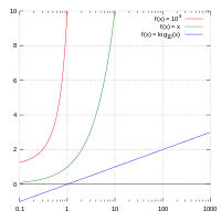
In science and engineering, a semi-log graph or semi-log plot is a way of visualizing data that are related according to an exponential relationship. One axis is plotted on a logarithmic scale. This kind of plot is useful when one of the variables being plotted covers a large range of values and the other has only a restricted range – the advantage being that it can bring out features in the data that would not easily be seen if both variables had been plotted linearly.[1]
All equations of the form  form straight lines when plotted semi-logarithmically, since taking logs of both sides gives

This can easily be seen as a line in slope-intercept form with  as the slope and
  as the vertical intercept. To facilitate use with logarithmic tables, one usually takes logs to base 10 or e, or sometimes base 2:

The term log-lin is used to describe a semi-log plot with a logarithmic scale on the y-axis, and a linear scale on the x-axis. Likewise, a lin-log plot uses a logarithmic scale on the x-axis, and a linear scale on the y-axis. Note that the naming is output-input (y-x), the opposite order from (x, y).
On a semi-log plot the spacing of the scale on the y-axis (or x-axis) is proportional to the logarithm of the number, not the number itself. It is equivalent to converting the y values (or x values) to their log, and plotting the data on lin-lin scales. A log-log plot uses the logarithmic scale for both axes, and hence is not a semi-log plot.
Equations
The equation for a line with an ordinate axis logarithmically scaled would be:


The equation of a line on a plot where the abscissa axis is scaled logarithmically would be
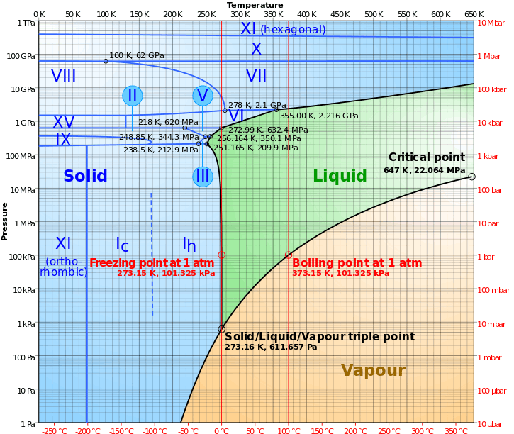
Real-world examples
Phase diagram of water
In physics and chemistry, a plot of logarithm of pressure against temperature can be used to illustrate the various phases of a substance, as in the following for water:
2009 "swine flu" progression
While ten is the most common base, there are times when other bases are more appropriate, as in this example:

Microbial growth
In biology and biological engineering, the change in numbers of microbes due to asexual reproduction and nutrient exhaustion is commonly illustrated by a semi-log plot. Time is usually the independent axis, with the logarithm of the number or mass of bacteria or other microbe as the dependent variable. This forms a plot with four distinct phases, as shown below.

See also
- Nomograph, more complicated graphs
- Nonlinear regression#Transformation, for converting a nonlinear form to a semi-log form amenable to non-iterative calculation