Nonlinear regression
| Part of a series on Statistics |
| Regression analysis |
|---|
 |
| Models |
| Estimation |
| Background |
|

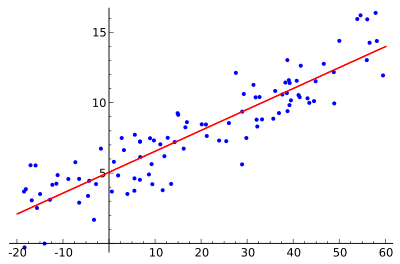
In statistics, nonlinear regression is a form of regression analysis in which observational data are modeled by a function which is a nonlinear combination of the model parameters and depends on one or more independent variables. The data are fitted by a method of successive approximations.
General
The data consist of error-free independent variables (explanatory variables), x, and their associated observed dependent variables (response variables), y. Each y is modeled as a random variable with a mean given by a nonlinear function f(x,β). Systematic error may be present but its treatment is outside the scope of regression analysis. If the independent variables are not error-free, this is an errors-in-variables model, also outside this scope.
For example, the Michaelis–Menten model for enzyme kinetics
can be written as
where is the parameter , is the parameter and [S] is the independent variable, x. This function is nonlinear because it cannot be expressed as a linear combination of the two s.
Other examples of nonlinear functions include exponential functions, logarithmic functions, trigonometric functions, power functions, Gaussian function, and Lorenz curves. Some functions, such as the exponential or logarithmic functions, can be transformed so that they are linear. When so transformed, standard linear regression can be performed but must be applied with caution. See Linearization, below, for more details.
In general, there is no closed-form expression for the best-fitting parameters, as there is in linear regression. Usually numerical optimization algorithms are applied to determine the best-fitting parameters. Again in contrast to linear regression, there may be many local minima of the function to be optimized and even the global minimum may produce a biased estimate. In practice, estimated values of the parameters are used, in conjunction with the optimization algorithm, to attempt to find the global minimum of a sum of squares.
For details concerning nonlinear data modeling see least squares and non-linear least squares.
Regression statistics
The assumption underlying this procedure is that the model can be approximated by a linear function.
where . It follows from this that the least squares estimators are given by
The nonlinear regression statistics are computed and used as in linear regression statistics, but using J in place of X in the formulas. The linear approximation introduces bias into the statistics. Therefore more caution than usual is required in interpreting statistics derived from a nonlinear model.
Ordinary and weighted least squares
The best-fit curve is often assumed to be that which minimizes the sum of squared residuals. This is the (ordinary) least squares (OLS) approach. However, in cases where the dependent variable does not have constant variance, a sum of weighted squared residuals may be minimized; see weighted least squares. Each weight should ideally be equal to the reciprocal of the variance of the observation, but weights may be recomputed on each iteration, in an iteratively weighted least squares algorithm.
Linearization
Transformation
Some nonlinear regression problems can be moved to a linear domain by a suitable transformation of the model formulation.
For example, consider the nonlinear regression problem
with parameters a and b and with multiplicative error term U. If we take the logarithm of both sides, this becomes
where u = ln(U), suggesting estimation of the unknown parameters by a linear regression of ln(y) on x, a computation that does not require iterative optimization. However, use of a nonlinear transformation requires caution. The influences of the data values will change, as will the error structure of the model and the interpretation of any inferential results. These may not be desired effects. On the other hand, depending on what the largest source of error is, a nonlinear transformation may distribute your errors in a normal fashion, so the choice to perform a nonlinear transformation must be informed by modeling considerations.
For Michaelis–Menten kinetics, the linear Lineweaver–Burk plot
of 1/v against 1/[S] has been much used. However, since it is very sensitive to data error and is strongly biased toward fitting the data in a particular range of the independent variable, [S], its use is strongly discouraged.
For error distributions that belong to the exponential family, a link function may be used to transform the parameters under the Generalized linear model framework.
Segmentation

The independent or explanatory variable (say X) can be split up into classes or segments and linear regression can be performed per segment. Segmented regression with confidence analysis may yield the result that the dependent or response variable (say Y) behaves differently in the various segments.[1]
The figure shows that the soil salinity (X) initially exerts no influence on the crop yield (Y) of mustard (colza), until a critical or threshold value (breakpoint), after which the yield is affected negatively.[2]
See also
References
- ↑ R.J.Oosterbaan, 1994, Frequency and Regression Analysis. In: H.P.Ritzema (ed.), Drainage Principles and Applications, Publ. 16, pp. 175-224, International Institute for Land Reclamation and Improvement (ILRI), Wageningen, The Netherlands. ISBN 90-70754-33-9 . Download as PDF :
- ↑ R.J.Oosterbaan, 2002. Drainage research in farmers' fields: analysis of data. Part of project “Liquid Gold” of the International Institute for Land Reclamation and Improvement (ILRI), Wageningen, The Netherlands. Download as PDF : . The figure was made with the SegReg program, which can be downloaded freely from
Further reading
- Bethea, R. M.; Duran, B. S.; Boullion, T. L. (1985). Statistical Methods for Engineers and Scientists. New York: Marcel Dekker. ISBN 0-8247-7227-X.
- Meade, N.; Islam, T. (1995). "Prediction Intervals for Growth Curve Forecasts". Journal of Forecasting. 14 (5): 413–430. doi:10.1002/for.3980140502.
- Schittkowski, K. (2002). Data Fitting in Dynamical Systems. Boston: Kluwer. ISBN 1402010796.
- Seber, G. A. F.; Wild, C. J. (1989). Nonlinear Regression. New York: John Wiley and Sons. ISBN 0471617601.