Shear stress
| Shear stress | |
|---|---|
Common symbols | τ |
| SI unit | pascal |
Derivations from other quantities | τ = F/A |
A shear stress, often denoted τ (Greek: tau), is defined as the component of stress coplanar with a material cross section. Shear stress arises from the force vector component parallel to the cross section. Normal stress, on the other hand, arises from the force vector component perpendicular to the material cross section on which it acts.
General shear stress
The formula to calculate average shear stress is force per unit area.:[1]

where:
- τ = the shear stress;
- F = the force applied;
- A = the cross-sectional area of material with area parallel to the applied force vector.
Other forms
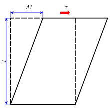
Pure
Pure shear stress is related to pure shear strain, denoted γ, by the following equation:[2]

where G is the shear modulus of the isotropic material, given by

Here E is Young's modulus and ν is Poisson's ratio.
Beam shear
Beam shear is defined as the internal shear stress of a beam caused by the shear force applied to the beam.

where
- V = total shear force at the location in question;
- Q = statical moment of area;
- t = thickness in the material perpendicular to the shear;
- I = Moment of Inertia of the entire cross sectional area.
The beam shear formula is also known as Zhuravskii shear stress formula after Dmitrii Ivanovich Zhuravskii who derived it in 1855.[3][4]
Semi-monocoque shear
Shear stresses within a semi-monocoque structure may be calculated by idealizing the cross-section of the structure into a set of stringers (carrying only axial loads) and webs (carrying only shear flows). Dividing the shear flow by the thickness of a given portion of the semi-monocoque structure yields the shear stress. Thus, the maximum shear stress will occur either in the web of maximum shear flow or minimum thickness
Also constructions in soil can fail due to shear; e.g., the weight of an earth-filled dam or dike may cause the subsoil to collapse, like a small landslide.
Impact shear
The maximum shear stress created in a solid round bar subject to impact is given as the equation:

where
- U = change in kinetic energy;
- G = shear modulus;
- V = volume of rod;
and
- U = Urotating + Uapplied;
- Urotating = 1/2Iω2;
- Uapplied = Tθdisplaced;
- I = mass moment of inertia;
- ω = angular speed.
Shear stress in fluids
Any real fluids (liquids and gases included) moving along solid boundary will incur a shear stress on that boundary. The no-slip condition[5] dictates that the speed of the fluid at the boundary (relative to the boundary) is zero, but at some height from the boundary the flow speed must equal that of the fluid. The region between these two points is aptly named the boundary layer. For all Newtonian fluids in laminar flow the shear stress is proportional to the strain rate in the fluid where the viscosity is the constant of proportionality. However, for non-Newtonian fluids, this is no longer the case as for these fluids the viscosity is not constant. The shear stress is imparted onto the boundary as a result of this loss of velocity. The shear stress, for a Newtonian fluid, at a surface element parallel to a flat plate, at the point y, is given by:

where
- μ is the dynamic viscosity of the flow;
- u is the flow velocity along the boundary;
- y is the height above the boundary.
Specifically, the wall shear stress is defined as:

The Newton's constitutive law, for any general geometry (including the flat plate above mentioned), states that shear tensor (a second-order tensor) is proportional to the flow velocity gradient (the velocity is a vector, so its gradient is a second-order tensor):

and the constant of proportionality is named dynamic viscosity. For an isotropic Newtonian flow it is a scalar, while for anisotropic Newtonian flows it can be a second-order tensor too. The fundamental aspect is that for a Newtonian fluid the dynamic viscosity is independent on flow velocity (i.e., the shear stress constituive law is linear), while non-Newtonian flows this is not true, and one should allow for the modification:

The above formula is no longer the Newton's law but a generic tensorial identity: one could always find an expression of the viscosity as function of the flow velocity given any expression of the shear stress as function of the flow velocity. On the other hand, given a shear stress as function of the flow velocity, it represents a Newtonian flow only if it can be expressed as a constant for the gradient of the flow velocity. The constant one finds in this case is the dynamic viscosity of the flow.
Example
Considering a 2D space in cartesian coordinates (x,y) (the flow velocity components are respectively (u,v)), the shear stress matrix given by:

represents a Newtonian flow, in fact it can be expressed as:
- ,

i.e., an anisotropic flow with the viscosity tensor:

which is nonuniform (depends on space coordinates) and transient, but relevantly it is independent on the flow velocity:

This flow is therefore newtonian. On the other hand, a flow in which the viscosity were:

is Nonnewtonian since the viscosity depends on flow velocity. This nonnewtonian flow is isotropic (the matrix is proportional to the identity matrix), so the viscosity is simply a scalar:
- .

Measurement with sensors
Diverging fringe shear stress sensor
This relationship can be exploited to measure the wall shear stress. If a sensor could directly measure the gradient of the velocity profile at the wall, then multiplying by the dynamic viscosity would yield the shear stress. Such a sensor was demonstrated by A. A. Naqwi and W. C. Reynolds.[6] The interference pattern generated by sending a beam of light through two parallel slits forms a network of linearly diverging fringes that seem to originate from the plane of the two slits (see double-slit experiment). As a particle in a fluid passes through the fringes, a receiver detects the reflection of the fringe pattern. The signal can be processed, and knowing the fringe angle, the height and velocity of the particle can be extrapolated. The measured value of wall velocity gradient is independent of the fluid properties and as a result does not require calibration. Recent advancements in the micro-optic fabrication technologies have made it possible to use integrated diffractive optical element to fabricate diverging fringe shear stress sensors usable both in air and liquid.[7]
Micro-pillar shear-stress sensor
A further technique is that of slender wall-mounted micro-pillars made of the flexible polymer PDMS, which bend in reaction to the applying drag forces in the vicinity of the wall. The sensor thereby belongs to the indirect measurement principles relying on the relationship between near-wall velocity gradients and the local wall-shear stress.[8][9]
See also
- Critical resolved shear stress
- Direct shear test
- Shear and moment diagrams
- Shear rate
- Shear strain
- Shear strength
- Tensile stress
- Triaxial shear test
References
- ↑ Hibbeler, R.C. (2004). Mechanics of Materials. New Jersey USA: Pearson Education. p. 32. ISBN 0-13-191345-X.
- ↑ "Strength of Materials". Eformulae.com. Retrieved 24 December 2011.
- ↑ Лекция Формула Журавского [Zhuravskii's Formula]. Сопромат Лекции (in Russian). Retrieved 2014-02-26.
- ↑ "Flexure of Beams" (PDF). Mechanical Engineering Lectures. McMaster University.
- ↑ Day, Michael A. (2004), The no-slip condition of fluid dynamics, Springer Netherlands, pp. 285–296, ISSN 0165-0106.
- ↑ Naqwi, A. A.; Reynolds, W. C. (Jan 1987), "Dual cylindrical wave laser-Doppler method for measurement of skin friction in fluid flow", NASA STI/Recon Technical Report N, 87
- ↑ {microS Shear Stress Sensor, MSE}
- ↑ Große, S.; Schröder, W. (2009), "Two-Dimensional Visualization of Turbulent Wall Shear Stress Using Micropillars", AIAA Journal, 47 (2): 314–321, Bibcode:2009AIAAJ..47..314G, doi:10.2514/1.36892
- ↑ Große, S.; Schröder, W. (2008), "Dynamic Wall-Shear Stress Measurements in Turbulent Pipe Flow using the Micro-Pillar Sensor MPS3", International Journal of Heat and Fluid Flow, 29 (3): 830–840, doi:10.1016/j.ijheatfluidflow.2008.01.008