Stretched grid method
The stretched grid method (SGM) is a numerical technique for finding approximate solutions of various mathematical and engineering problems that can be related to an elastic grid behavior. In particular, meteorologists use the stretched grid method for weather prediction[1] and engineers use the stretched grid method to design tents and other tensile structures.
FEM and BEM mesh refinement
In recent decades the finite element and boundary element methods (FEM and BEM) have become a mainstay for industrial engineering design and analysis. Increasingly larger and more complex designs are being simulated using the FEM or BEM. However, some problems of FEM and BEM engineering analysis are still on the cutting edge. The first problem is a reliability of engineering analysis that strongly depends upon the quality of initial data generated at the pre-processing stage. It is known that automatic element mesh generation techniques at this stage have become commonly used tools for the analysis of complex real-world models.[2] With FEM and BEM increasing in popularity comes the incentive to improve automatic meshing algorithms. However, all of these algorithms can create distorted and even unusable grid elements. Several techniques exist which can take an existing mesh and improve its quality. For instance smoothing (also referred to as mesh refinement) is one such method, which repositions nodal locations, so as to minimize element distortion. The Stretched Grid Method (SGM) allows the obtaining of pseudo-regular meshes very easily and quickly in a one-step solution(see [3]).
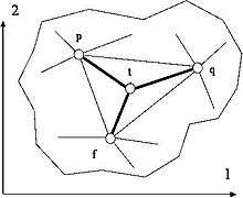
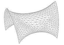
Let one assume that there is an arbitrary triangle grid embedded into plane polygonal single-coherent contour and produced by an automeshing procedure (see fig. 1) It may be assumed further that the grid considered as a physical nodal system is distorted by a number of distortions. It is supposed that the total potential energy of this system is proportional to the length of some  -dimensional vector with all network segments as its components.
Thus, the potential energy takes the following form
where
- - total number of segments in the network,
 - The length of segment number
  ,
, - an arbitrary constant.
The length of segment number may be expressed by two nodal co-ordinates as
It may also be supposed that co-ordinate vector  of all nodes is associated with non-distorted network and co-ordinate vector
  is associated with the distorted network. The expression for vector may be written as

The vector determination is related to minimization of the quadratic form  by incremental vector
  , i.e.

where
 - is the number of interior node of the area,
 - the number of co-ordinate
After all transformations we may write the following two independent systems of linear algebraic equations
![[\ A] \{\Delta X_1\} = \{\ B_1\}](../I/m/8bf79ac98e196b5c888569a4523d8f64.png)
![[\ A] \{\Delta X_2\} = \{\ B_2\}](../I/m/f0db0a4e92bdd3063405975fe531c811.png)
where
![[\ A]](../I/m/6292c2c690956c1405b435d2abfc9c1b.png) - symmetrical matrix in the banded form similar to global stiffness matrix of FEM assemblage,
- symmetrical matrix in the banded form similar to global stiffness matrix of FEM assemblage, and
and  - incremental vectors of co-ordinates of all nodes at axes 1, 2,
 and
and  - the right part vectors that are combined by co-ordinates of all nodes in axes 1, 2.
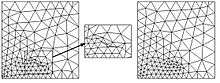
The solution of both systems, keeping all boundary nodes conservative, obtains new interior node positions corresponding to a non-distorted mesh with pseudo-regular elements. For example, Fig. 2 presents the rectangular area covered by a triangular mesh. The initial auto mesh possesses some degenerative triangles (left mesh). The final mesh (right mesh) produced by the SGM procedure is pseudo-regular without any distorted elements.
As above systems are linear, the procedure elapses very quickly to a one-step solution. Moreover, each final interior node position meets the requirement of co-ordinate arithmetic mean of nodes surrounding it and meets the Delaunay criteria too. Therefore, the SGM has all the positive values peculiar to Laplacian and other kinds of smoothing approaches but much easier and reliable because of integer-valued final matrices representation. Finally, the described above SGM is perfectly applicable not only to 2D meshes but to 3D meshes consisting of any uniform cells as well as to mixed or transient meshes.
Minimum surface problem solution
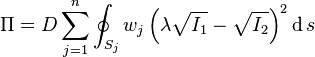
Mathematically the surface embedded into a non-plane closed curve is called minimum if its area is minimal amongst all the surfaces passing through this curve. The best-known minimum surface sample is a soap film bounded by wire frame. Usually to create a minimum surface, a fictitious constitutive law, which maintains a constant prestress, independent of any changes in strain, is used.[4] The alternative approximated approach to the minimum surface problem solution is based on SGM. This formulation allows one to minimize the surface embedded into non-plane and plane closed contours.

The idea is to approximate a surface part embedded into 3D non-plane contour by an arbitrary triangle grid. To converge such triangle grid to grid with minimum area one should solve the same two systems described above. Increments of the third nodal co-ordinates may be determined additionally by similar system at axis 3 in the following way
![[\ A] \{\Delta X_3\} = \{\ B_3\}](../I/m/f984a80eb995a8115d3b36523db1dc6c.png)
Solving all three systems simultaneously one can obtain a new grid that will be the approximating minimal surface embedded into non-plane closed curve because of the minimum of the function where parameter  .
.
As an example the surface of catenoid which is calculated by the described above approach is presented in Fig 3. The radii of rings and the height of catenoid are equal to 1.0. The numerical area of catenoidal surface determined by SGM is equal to 2,9967189 (exact value is 2.992).
Tensile fabric structures form finding
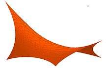
For structural analysis, the configuration of the structure is generally known à priori. This is not the case for tensile structures such as tension fabric structures. Since the membrane in a tension structure possesses no flexural stiffness, its form or configuration depends upon initial prestressing and the loads to which it is subjected. Thus, the load-bearing behaviour and the shape of the membrane cannot be separated and cannot be generally described by simple geometric models only. The membrane shape, the loads on the structure and the internal stresses interact in a non-linear manner to satisfy the equilibrium equations.

The preliminary design of tension structures involves the determination of an initial configuration referred to as form finding. In addition to satisfying the equilibrium conditions, the initial configuration must accommodate both architectural (aesthetics) and structural (strength and stability) requirements. Further, the requirements of space and clearance should be met, the membrane principal stresses must be tensile to avoid wrinkling, and the radii of the double-curved surface should be small enough to resist out-of-plane loads and to insure structural stability (work [5]). Several variations on form finding approaches based on FEM have been developed to assist engineers in the design of tension fabric structures. All of them are based on the same assumption as that used for analysing the behaviour of tension structures under various loads. However, as it is noted by some researchers it might sometimes be preferable to use the so-called ‘minimal surfaces’ in the design of tension structures.
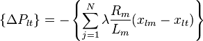
The physical meaning of SGM consists in convergence of the energy of an arbitrary grid structure embedded into rigid (or elastic) 3D contour to minimum that is equivalent to minimum sum distances between arbitrary pairs of grid nodes. It allows the minimum surface energy problem solution substituting for finding grid structure sum energy minimum finding that provides much more plain final algebraic equation system than the usual FEM formulation. The generalized formulation of SGM presupposes a possibility to apply a set of outer forces and rigid or elastic constrains to grid structure nodes that allows the modelling of various outer effects. We may obtain the following expression for such SGM formulation
where
- - total number of grid segments,
 - total number of nodes,
- - length of segment number ,
 - stiffness of segment number ,
 - coordinate increment of node at axis
  ,
, - stiffness of an elastic constrain in node at axis ,
 - outer force in node at axis .
Unfolding problem and cutting pattern generation
Once a satisfactory shape has been found, a cutting pattern may be generated. Tension structures are highly varied in their size, curvature and material stiffness. Cutting pattern approximation is strongly related to each of these factors. It is essential for a cutting pattern generation method to minimize possible approximation and to produce reliable plane cloth data.
The objective is to develop the shapes described by these data, as close as possible to the ideal doubly curved strips. In general, cutting pattern generation involves two steps. First, the global surface of a tension structure is divided into individual cloths. The corresponding cutting pattern at the second step can be found by simply taking each cloth strip and unfolding it on a planar area. In the case of the ideal doubly curved membrane surface the subsurface cannot be simply unfolded and they must be flattened. For example, in,[6][7] SGM has been used for the flattening problem solution.
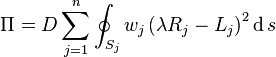
The cutting pattern generation problem is actually subdivided into two independent formulations. These are the generation of a distortion-free plane form unfolding each cloth strip and flattening double-curved surfaces that cannot be simply unfolded. Studying the problem carefully one can notice that from the position of differential geometry both formulations are the same. We may consider it as an isometric mapping of a surface onto the plane area that will be conformal mapping and equiareal mapping simultaneously because of invariant angles between any curves and invariance of any pieces of area. In the case of single-curved surface that can be unfolded precisely equi-areal mapping allows one to obtain a cutting pattern for fabric structure without any distortions. The second type of surfaces can be equi-areal mapped only approximately with some distortions of linear surface elements limited by the fabric properties. Let us assume that two surfaces are parameterized so that their first quadratic forms may be written as follows


The condition of conformal mapping for two surfaces as is formulated in differential geometry requires that

where  is the ratio of the surface distortion due to conformal mapping.
It is known that the first quadratic form reflects the distance between two surface points  and
and  . When -ratio is close to 1 the above eqn converges to condition of isometric mapping and to equi-areal mapping respectively because of invariant angles between any curves and invariance of any pieces of area. Remembering that the first stage of form finding is based on triangular mesh of a surface and using the method of weighted residuals for the description of isometric and equi-areal mapping of the minimum surface onto a plane area we may write the following function which is defined by the sum of integrals along segments of curved triangles
where
- - total number of grid cells,
 - weight ratios,
- - the total mapping residual,
- - the constant that does not influence the final result and may be used as a scale ratio.
Considering further weight ratios  we may transform eqn. into approximate finite sum that is a combination of linear distances between nodes of the surface grid and write the basic condition of equi-areal surface mapping as a minimum of following non-linear function
where
- - initial length of linear segment number ,
 - final length of segment number ,
- - distortion ratio close to 1 and may be different for each segment.
The initial and final lengths of segment number may be expressed as usual by two nodal co-ordinates as

where
 - co-ordinates of nodes of the initial segment,
 - co-ordinates of nodes of the final segment.
According to the initial assumption we can write  for the plane surface mapping. The expression for vectors
  and with co-ordinate increments term use may be written as


The vector definition is made as previously
After transformations we may write the following two independent systems of non-linear algebraic equations
![[\ A] \{\Delta X_1\} = \{\ B_1\} + \{\Delta P_1\}](../I/m/c138d45f46cfdd2b21cdf9238a3e4093.png)
![[\ A] \{\Delta X_2\} = \{\ B_2\} + \{\Delta P_2\}](../I/m/ee8419b2cd82747a32d0e7a731b15e7e.png)
where all the parts of the system can be expressed as previously and  and
and  are vectors of pseudo-stresses at axes 1, 2 that has the following form
where
 - total number of nodes that surround node number
  ,
,- - the number of global axes.
The above approach is another form of SGM and allows the obtaining of two independent systems of non-linear algebraic equations that can be solved by any standard iteration procedure. The less Gaussian curvature of the surface is the higher the accuracy of the plane mapping is. As a rule, the plane mapping allows to obtain a pattern with linear dimensions 1–2% less than corresponding spatial lines of a final surface. That is why it is necessary to provide the appropriate margins while patterning.
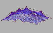
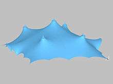
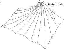
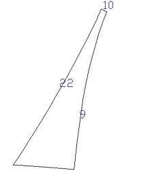
The typical sample of cut out — also called a cutout, a gore (segment), or a patch — is presented in Figs. 9, 10, 11.
References
- ↑ QIAN Jian-hua. "Application of a Variable-Resolution Stretched Grid to a Regional Atmospheric Model with Physics Parameterization"
- ↑ Zienkiewicz O. C., Kelly D.W., Bettes P. The coupling of the finite element method and boundary solution procedure. // International journal of Numerical Methods in Engineering, vol. 11, N 12, 1977. pp. 355–375.
- ↑ Popov E.V.,On Some Variational Formulations for Minimum Surface. Transactions of Canadian Society of Mechanics for Engineering, Univ. of Alberta, vol.20, N 4, 1997, pp. 391–400.
- ↑ Tabarrok, Y.Xiong. Some Variational Formulations for minimum surface. Acta Mechanica, vol.89/1–4, 1991, pp. 33–43.
- ↑ B.Tabarrok, Z.Qin. Form Finding and Cutting Pattern Generation for Fabric Tension Structures, -Microcomputers in Civil Engineering J., № 8, 1993, pp. 377–384).
- ↑ Popov E.V. Geometrical Modeling of Tent Fabric Structures with the Stretched Grid Method. (written in Russian) Proceedings of the 11th International Conference on Computer Graphics&Vision GRAPHICON’2001, UNN, Nizhny Novgorod, 2001. pp. 138–143.
- ↑ Popov, E.V. Cutting pattern generation for tent type structures represented by minimum surfaces. The Transactions of the Canadian Society for Mechanical Engineering, Univ. of Alberta, vol. 22, N 4A, 1999, pp. 369–377.