Transformation between distributions in time–frequency analysis
In the field of time–frequency analysis, several signal formulations are used to represent the signal in a joint time–frequency domain.[1]
There are several methods and transforms called "time-frequency distributions" (TFDs), whose interconnections were organized by Leon Cohen.[2] [3][4][5] The most useful and popular methods form a class referred to as "quadratic" or bilinear time–frequency distributions. A core member of this class is the Wigner–Ville distribution (WVD), as all other TFDs can be written as a smoothed or convolved versions of the WVD. Another popular member of this class is the spectrogram which is the square of the magnitude of the short-time Fourier transform (STFT). The spectrogram has the advantage of being positive and is easy to interpret, but also has disadvantages, like being irreversible, which means that once the spectrogram of a signal is computed, the original signal can't be extracted from the spectrogram. The theory and methodology for defining a TFD that verifies certain desirable properties is given in the "Theory of Quadratic TFDs".[6]
The scope of this article is to illustrate some elements of the procedure to transform one distribution into another. The method used to transform a distribution is borrowed from the phase space formulation of quantum mechanics, even though the subject matter of this article is "signal processing". Noting that a signal can recovered from a particular distribution under certain conditions, given a certain TFD ρ1(t,f) representing the signal in a joint time–frequency domain, another, different, TFD ρ2(t,f) of the same signal can be obtained to calculate any other distribution, by simple smoothing or filtering; some of these relationships are shown below. A full treatment of the question can be given in Cohen's book.
General class
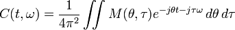
If we use the variable ω=2πf, then, borrowing the notations used in the field of quantum mechanics, we can show that time–frequency representation, such as Wigner distribution function (WDF) and other bilinear time–frequency distributions, can be expressed as
-
 (1)
(1)
where  is a two dimensional function called the kernel, which determines the distribution and its properties (for a signal processing terminology and treatment of this question, the reader is referred to the references already cited in the introduction).
The kernel of the Wigner distribution function (WDF) is one. However, no particular significance should be attached to that, since it is possible to write the general form so that the kernel of any distribution is one, in which case the kernel of the Wigner distribution function (WDF) would be something else.
Characteristic function formulation
The characteristic function is the double Fourier transform of the distribution. By inspection of Eq. (1), we can obtain that
-
 (2)
(2)
where
-
 (3)
(3)
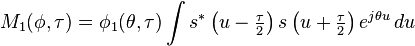
and where  is the symmetrical ambiguity function. The characteristic function may be appropriately called the generalized ambiguity function.
Transformation between distributions
To obtain that relationship suppose that there are two distributions,  and
and  , with corresponding kernels,
  and
and  . Their characteristic functions are
-
 (4)
(4)
-
 (5)
(5)
Divide one equation by the other to obtain
-
 (6)
(6)
This is an important relationship because it connects the characteristic functions. For the division to be proper the kernel cannot to be zero in a finite region.
To obtain the relationship between the distributions take the double Fourier transform of both sides and use Eq. (2)
-
 (7)
(7)
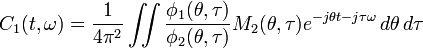
Now express  in terms of to obtain
-
 (8)
(8)
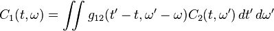
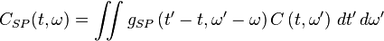
This relationship can be written as
-
 (9)
(9)
with
-
 (10)
(10)
Relation of the spectrogram to other bilinear representations
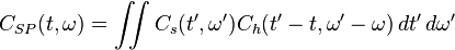
Now we specialize to the case where one transform from an arbitrary representation to the spectrogram. In Eq. (9), both to be the spectrogram and to be arbitrary are set. In addition, to simplify notation, 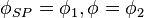 , and
, and  are set and written as
-
 (11)
(11)
The kernel for the spectrogram with window,  , is
, is  and therefore
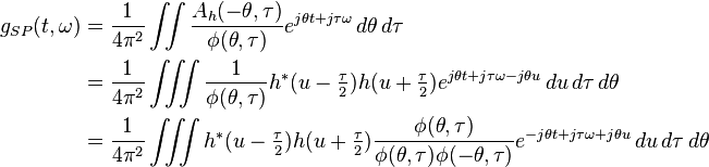
If we only consider kernels for which 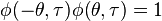 holds then

and therefore
This was shown by Janssen[4]. When 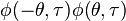 does not equal one, then

where

References
- ↑ L. Cohen, "Time–Frequency Analysis," Prentice-Hall, New York, 1995. ISBN 978-0135945322
- ↑ L. Cohen, "Generalized phase-space distribution functions," J. Math. Phys., 7 (1966) pp. 781–786, doi:10.1063/1.1931206
- ↑ L. Cohen, "Quantization Problem and Variational Principle in the Phase Space Formulation of Quantum Mechanics," J. Math. Phys., 7 pp. 1863–1866, 1976.
- ↑ A. J. E. M. Janssen, "On the locus and spread of pseudo-density functions in the time frequency plane," Philips Journal of Research, vol. 37, pp. 79–110, 1982.
- ↑ E. Sejdić, I. Djurović, J. Jiang, “Time-frequency feature representation using energy concentration: An overview of recent advances,” Digital Signal Processing, vol. 19, no. 1, pp. 153-183, January 2009.
- ↑ B. Boashash, “Theory of Quadratic TFDs”, Chapter 3, pp. 59–82, in B. Boashash, editor, Time-Frequency Signal Analysis & Processing: A Comprehensive Reference, Elsevier, Oxford, 2003; ISBN 0-08-044335-4.