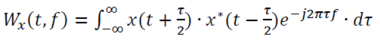
Wigner distribution function

Wigner Ville (top) vs FIR bank (bottom) time-frequency distribution analysis. The Wigner Ville spectrogram contains less frequency uncertainty on the Y axis, and it contains more artefacts, a lower resolution, and an increased computing time, compared to an array of BP2 filters displayed in green.

The Wigner distribution function (WDF) is used in signal processing as a transform in time-frequency analysis.

The WDF was first proposed in physics to account for quantum corrections to classical statistical mechanics in 1932 by Eugene Wigner, and it is of importance in quantum mechanics in phase space (see, by way of comparison: Wigner quasi-probability distribution, also called the Wigner function or the Wigner–Ville distribution).

Given the shared algebraic structure between position-momentum and time-frequency conjugate pairs, it also usefully serves in signal processing, as a transform in time-frequency analysis, the subject of this article. Compared to a short-time Fourier transform, such as the Gabor transform, the Wigner distribution function can furnish higher clarity in some cases.

Mathematical definition

There are several different definitions for the Wigner distribution function. The definition given here is specific to time-frequency analysis. Given the time series $x[t]$ , its non-stationary autocorrelation function is given by

C_x(t_1, t_2) = \left\langle \left(x[t_1] - \mu[t_1]\right) \left(x[t_2] - \mu[t_2]\right)^* \right\rangle ,

where $\langle \cdots \rangle$ denotes the average over all possible realizations of the process and $\mu (t)$ is the mean, which may or may not be a function of time. The Wigner function $W_{x}(t,f)$ is then given by first expressing the autocorrelation function in terms of the average time $t=(t_{1}+t_{2})/2$ and time lag $\tau =t_{1}-t_{2}$ , and then Fourier transforming the lag.

W_x(t,f)=\int_{-\infty}^{\infty} C_x\left(t + \frac{\tau}{2}, t - \frac{\tau}{2}\right) \, e^{-2\pi i\tau f} \, d\tau .

So for a single (mean-zero) time series, the Wigner function is simply given by

W_x(t,f)=\int_{-\infty}^{\infty}x\left(t + \frac{\tau}{2}\right) \, x\left(t - \frac{\tau}{2}\right)^* \, e^{-2\pi i\tau f}\,d\tau .

The motivation for the Wigner function is that it reduces to the spectral density function at all times $t$ for stationary processes, yet it is fully equivalent to the non-stationary autocorrelation function. Therefore, the Wigner function tells us (roughly) how the spectral density changes in time.

Time-frequency analysis example

Here are some examples illustrating how the WDF is used in time-frequency analysis.

Constant input signal

When the input signal is constant, its time-frequency distribution is a horizontal line along the time axis. For example, if x(t) = 1, then

W_{x}(t,f)=\int _{{-\infty }}^{\infty }e^{{-i2\pi \tau \,f}}\,d\tau =\delta (f).

Sinusoidal input signal

When the input signal is a sinusoidal function, its time-frequency distribution is a horizontal line parallel to the time axis, displaced from it by the sinusoidal signal's frequency. For example, if $x (t) = e i2π kt$ , then

\begin{align} W_x(t,f) &= \int_{-\infty}^{\infty}e^{ i2\pi k \left(t + \frac{\tau}{2}\right)}e^{-i2\pi k\left(t - \frac{\tau}{2}\right)}e^{-i2\pi\tau\,f}\,d\tau \\ &= \int_{-\infty}^{\infty}e^{-i2\pi \tau \left(f - k\right)}\,d\tau\\ &= \delta(f - k). \end{align}

Chirp input signal

When the input signal is a linear chirp function, the instantaneous frequency is a linear function. This means that the time frequency distribution should be a straight line. For example, if

x(t) = e^{i2\pi kt^2}

then its instantaneous frequency is

\frac{1}{2\pi}\frac{d(2\pi kt^2)}{dt} = 2kt~,

and its WDF

\begin{align} W_x(t,f) &= \int_{-\infty}^\infty e^{i2\pi k\left(t + \frac{\tau}{2}\right)^2}e^{-i2\pi k\left(t - \frac{\tau}{2}\right)^2}e^{-i2\pi\tau\,f} \, d\tau \\ &= \int_{-\infty}^\infty e^{i4\pi kt\tau}e^{-i2\pi\tau f}\,d\tau \\ &= \int_{-\infty}^\infty e^{-i2\pi\tau(f - 2kt)}\,d\tau\\ &= \delta(f - 2kt) ~. \end{align}

Delta input signal

When the input signal is a delta function, since it is only non-zero at t=0 and contains infinite frequency components, its time-frequency distribution should be a vertical line across the origin. This means that the time frequency distribution of the delta function should also be a delta function. By WDF

{\begin{aligned}W_{x}(t,f)&=\int _{-\infty }^{\infty }\delta \left(t+{\frac {\tau }{2}}\right)\delta \left(t-{\frac {\tau }{2}}\right)e^{-i2\pi \tau \,f}\,d\tau \\&=4\int _{-\infty }^{\infty }\delta (2t+\tau )\delta (2t-\tau )e^{-i2\pi \tau f}\,d\tau \\&=4\delta (4t)e^{i4\pi tf}\\&=\delta (t)e^{i4\pi tf}\\&=\delta (t).\end{aligned}}

The Wigner distribution function is best suited for time-frequency analysis when the input signal's phase is 2nd order or lower. For those signals, WDF can exactly generate the time frequency distribution of the input signal.

Boxcar function

x(t) = \begin{cases} 1 & |t|<1/2 \\ 0 & \text{otherwise} \end{cases} \qquad

the rectangular function ⇒

W_{x}(t,f)={\begin{cases}{\frac {1}{\pi f}}\sin(2\pi f\{1-2|t|\})&|t|<1/2\\0&{\mbox{otherwise}}\end{cases}}

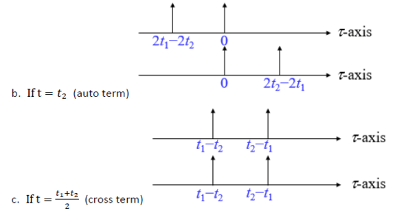
Cross term property

The Wigner distribution function is not a linear transform. A cross term ("time beats") occurs when there is more than one component in the input signal, analogous in time to frequency beats. In the ancestral physics Wigner quasi-probability distribution, this term has important and useful physics consequences, required for faithful expectation values. By contrast, the short-time Fourier transform does not have this feature. The following are some examples that exhibit the cross-term feature of the Wigner distribution function.

$x(t)={\begin{cases}\cos(2\pi t)&t\leq -2\\\cos(4\pi t)&-2<t\leq 2\\\cos(3\pi t)&t>2\end{cases}}$

$x(t)=e^{{it^{3}}}$

In order to reduce the cross term problem, many other transforms have been proposed, including the modified Wigner distribution function, the Gabor–Wigner transform, and Cohen’s class distribution.

Properties of the Wigner distribution function

The Wigner distribution function has several evident properties listed in the following table.

Projection property: $\begin{align} |x(t)|^2 &= \int_{-\infty}^\infty W_x(t,f)\,df \\ |X(f)|^2 &= \int_{-\infty}^\infty W_x(t,f)\,dt \end{align}$
Energy property: $\int _{{-\infty }}^{\infty }\int _{{-\infty }}^{\infty }W_{x}(t,f)\,df\,dt=\int _{{-\infty }}^{\infty }|x(t)|^{2}\,dt=\int _{{-\infty }}^{\infty }|X(f)|^{2}\,df$
Recovery property: $\begin{align} \int_{-\infty}^\infty W_x\left(\frac{t}{2}, f\right) e^{i2\pi ft}\,df &= x(t)x^*(0) \\ \int_{-\infty}^\infty W_x\left(t, \frac{f}{2}\right) e^{i2\pi ft}\,dt &= X(f)X^*(0) \end{align}$
Mean condition frequency and mean condition time: $\begin{align} X(f) &= |X(f)|e^{i2\pi\psi(f)},\quad x(t)=|x(t)|e^{i2\pi\phi(t)}, \\ \text{if } \phi'(t) &= |x(t)|^{-2}\int_{-\infty}^\infty fW_x(t,f)\,df \\ \text{ and } -\psi'(f) &= |X(f)|^{-2}\int_{-\infty}^\infty tW_x(t,f)\,dt \end{align}$
Moment properties: $\begin{align} \int_{-\infty}^\infty \int_{-\infty}^\infty t^nW_x(t,f)\,dt\,df &= \int_{-\infty}^\infty t^n|x(t)|^2\,dt \\ \int_{-\infty}^\infty \int_{-\infty}^\infty f^nW_x(t,f)\,dt\,df &= \int_{-\infty}^\infty f^n|X(f)|^2\,df \end{align}$
Real properties: $W^*_x(t, f) = W_x(t, f)$
Region properties: $\begin{align} \text{If } x(t) &= 0 \text{ for } t > t_0 \text{ then } W_x(t, f) = 0 \text{ for } t > t_0 \\ \text{If } x(t) &= 0 \text{ for } t < t_0 \text{ then } W_x(t, f) = 0 \text{ for } t < t_0 \end{align}$
Multiplication theorem: ${\begin{aligned}{\text{If }}y(t)&=x(t)h(t)\\{\text{then }}W_{y}(t,f)&=\int _{-\infty }^{\infty }W_{x}(t,\rho )W_{h}(t,f-\rho )\,d\rho \end{aligned}}$
Convolution theorem: $\begin{align} \text{If } y(t) &= \int_{-\infty}^\infty x(t - \tau)h(\tau)\,d\tau\\ \text{then } W_y(t, f) &= \int_{-\infty}^\infty W_x(\rho, f)W_h(t - \rho, f)\,d\rho \end{align}$
Correlation theorem: $\begin{align} \text{If } y(t) &= \int_{-\infty}^\infty x(t + \tau)h^*(\tau)\,d\tau\text{ then } \\ W_y(t, \omega) &= \int_{-\infty}^\infty W_x(\rho,\omega)W_h(-t + \rho, \omega)\,d\rho \end{align}$
Time-shifting covariance: $\begin{align} \text{If } y(t) &= x(t - t_0) \\ \text{then } W_y(t,f) &= W_x(t - t_0, f) \end{align}$
Modulation covariance: $\begin{align} \text{If } y(t) &= e^{i2\pi f_0t}x(t) \\ \text{then } W_y(t, f) &= W_x(t, f - f_0) \end{align}$
Scale covariance: $\begin{align} \text{If } y(t) &= \sqrt{a} x(a t) \text{ for some } a > 0 \text{ then }\\ \text{then } W_y(t, f) &= W_x(at, \frac{f}{a}) \end{align}$

Windowed Wigner Distribution Function

When a signal is not time limited, its Wigner Distribution Function is hard to implement. Thus we add a new function(mask) to its integration part, so that we only have to implement part of the original function instead of integrate all the way from negative infinity to positive infinity. Original function:

Function with mask:

is real and time-limited

Advantages and disadvantages

Advantages

Reduces computation time.
May reduce the cross term problem, but not always.

Disadvantages

May not totally eliminate the cross term problem.
May not meet the definition of Power Spectral Density.
May lose some good mathematical properties.

Implementation

According to definition:

And then we compare the difference between two conditions.

3 Conditions

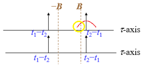
Then we consider the condition with mask function:

We can see that

have value only between –B to B, thus conducting with

can remove cross term of the function. But if x(t) is not a Delta function nor a narrow frequency function, instead, it is a function with wide frequency or ripple. The edge of the signal may still exist between –B and B, which still cause the cross term problem.

for example:

References

Wigner, E. (1932). "On the Quantum Correction for Thermodynamic Equilibrium". Physical Review. 40 (5): 749. Bibcode:1932PhRv...40..749W. doi:10.1103/PhysRev.40.749.
J. Ville, 1948. "Théorie et Applications de la Notion de Signal Analytique", Câbles et Transmission, 2, 61–74 .
T. A. C. M. Classen and W. F. G. Mecklenbrauker, 1980. “The Wigner distribution-a tool for time-frequency signal analysis; Part I,” Philips J. Res., vol. 35, pp. 217–250.
L. Cohen (1989): Proceedings of the IEEE 77 pp. 941-981, Time-frequency distributions---a review
L. Cohen, Time-Frequency Analysis, Prentice-Hall, New York, 1995. ISBN 978-0135945322
S. Qian and D. Chen, Joint Time-Frequency Analysis: Methods and Applications, Chap. 5, Prentice Hall, N.J., 1996.
B. Boashash, "Note on the Use of the Wigner Distribution for Time Frequency Signal Analysis", IEEE Transactions on Acoustics, Speech, and Signal Processing, Vol. 36, No. 9, pp. 1518–1521, Sept. 1988. doi:10.1109/29.90380. B. Boashash, editor,Time-Frequency Signal Analysis and Processing – A Comprehensive Reference, Elsevier Science, Oxford, 2003, ISBN 0-08-044335-4.
F. Hlawatsch, G. F. Boudreaux-Bartels: “Linear and quadratic time-frequency signal representation,” IEEE Signal Processing Magazine, pp. 21–67, Apr. 1992.
R. L. Allen and D. W. Mills, Signal Analysis: Time, Frequency, Scale, and Structure, Wiley- Interscience, NJ, 2004.
R.B. Pachori and A. Nishad, "Cross-terms reduction in Wigner-Ville distribution using tunable-Q wavelet transform", Signal Processing, vol. 120, pp. 288–304, 2016.
Jian-Jiun Ding, Time frequency analysis and wavelet transform class notes, the Department of Electrical Engineering, National Taiwan University (NTU), Taipei, Taiwan, 2015.

This article is issued from Wikipedia - version of the 10/7/2016. The text is available under the Creative Commons Attribution/Share Alike but additional terms may apply for the media files.