Alpha beta filter
An alpha beta filter (also called alpha-beta filter, f-g filter or g-h filter [1]) is a simplified form of observer for estimation, data smoothing and control applications. It is closely related to Kalman filters and to linear state observers used in control theory. Its principal advantage is that it does not require a detailed system model.
Filter equations
An alpha beta filter presumes that a system is adequately approximated by a model having two internal states, where the first state is obtained by integrating the value of the second state over time. Measured system output values correspond to observations of the first model state, plus disturbances. This very low order approximation is adequate for many simple systems, for example, mechanical systems where position is obtained as the time integral of velocity. Based on a mechanical system analogy, the two states can be called position x and velocity v. Assuming that velocity remains approximately constant over the small time interval ΔT between measurements, the position state is projected forward to predict its value at the next sampling time using equation 1.
Since velocity variable v is presumed constant, so its projected value at the next sampling time equals the current value.
If additional information is known about how a driving function will change the v state during each time interval, equation 2 can be modified to include it.
The output measurement is expected to deviate from the prediction because of noise and dynamic effects not included in the simplified dynamic model. This prediction error r is also called the residual or innovation, based on statistical or Kalman filtering interpretations
Suppose that residual r is positive. This could result because the previous x estimate was low, the previous v was low, or some combination of the two. The alpha beta filter takes selected alpha and beta constants (from which the filter gets its name), uses alpha times the deviation r to correct the position estimate, and uses beta times the deviation r to correct the velocity estimate. An extra ΔT factor conventionally serves to normalize magnitudes of the multipliers.
The corrections can be considered small steps along an estimate of the gradient direction. As these adjustments accumulate, error in the state estimates is reduced. For convergence and stability, the values of the alpha and beta multipliers should be positive and small:[2]
Noise is suppressed only if , otherwise the noise is amplified.
Values of alpha and beta typically are adjusted experimentally. In general, larger alpha and beta gains tend to produce faster response for tracking transient changes, while smaller alpha and beta gains reduce the level of noise in the state estimates. If a good balance between accurate tracking and noise reduction is found, and the algorithm is effective, filtered estimates are more accurate than the direct measurements. This motivates calling the alpha-beta process a filter.
Algorithm Summary
Initialize.
- Set the initial values of state estimates x and v, using prior information or additional measurements; otherwise, set the initial state values to zero.
- Select values of the alpha and beta correction gains.
Update. Repeat for each time step ΔT:
  Project state estimates x and v using equations 1 and 2
  Obtain a current measurement of the output value
  Compute the residual r using equation 3
  Correct the state estimates using equations 4 and 5
  Send updated x and optionally v as the filter outputs
Sample Program
Alpha Beta filter can be implemented in C[3] as follows:
#include<stdio.h>
#include<stdlib.h>

int main()
{
	float dt = 0.5;
	float xk_1 = 0, vk_1 = 0, a = 0.85, b = 0.005;

	float xk, vk, rk;
	float xm;

	while( 1 )
	{
		xm = rand() % 100;// input signal

		xk = xk_1 + ( vk_1 * dt );
		vk = vk_1;

		rk = xm - xk;

		xk += a * rk;
		vk += ( b * rk ) / dt;

		xk_1 = xk;
		vk_1 = vk;

		printf( "%f \t %f\n", xm, xk_1 );
		sleep( 1 );
	}
}
Result
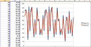
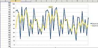
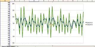
The following images depict the outcome of the above program in graphical format. In each image, the blue trace is the input signal; the output is red in the first image, yellow in the second, and green in the third. For the first two images, the output signal is visibly smoother than the input signal and lacks extreme spikes seen in the input. Also, the output moves in an estimate of gradient direction of input.
The higher the alpha parameter, the higher is the effect of input x and the less damping is seen. A low value of beta is effective in controlling sudden surges in velocity. Also, as alpha increases beyond unity, the output becomes rougher and more uneven than the input.[3]
 Results for alpha = 0.85 and beta = 0.005 |
 Results for alpha = 0.5 and beta = 0.1 |
 Results for alpha = 1.5 and beta = 0.5 |
Relationship to general state observers
More general state observers, such as the Luenberger observer for linear control systems, use a rigorous system model. Linear observers use a gain matrix to determine state estimate corrections from multiple deviations between measured variables and predicted outputs that are linear combinations of state variables. In the case of alpha beta filters, this gain matrix reduces to two terms. There is no general theory for determining the best observer gain terms, and typically gains are adjusted experimentally for both.
The linear Luenberger observer equations reduce to the alpha beta filter by applying the following specializations and simplifications.
- The discrete state transition matrix A is a square matrix of dimension 2, with all main diagonal terms equal to 1, and the first super-diagonal terms equal to ΔT.
- The observation equation matrix C has one row that selects the value of the first state variable for output.
- The filter correction gain matrix L has one column containing the alpha and beta gain values.
- Any known driving signal for the second state term is represented as part of the input signal vector u, otherwise the u vector is set to zero.
- Input coupling matrix B has a non-zero gain term as its last element if vector u is non-zero.
Relationship to Kalman Filters
A Kalman filter estimates the values of state variables and corrects them in a manner similar to an alpha beta filter or a state observer. However, a Kalman filter does this in a much more formal and rigorous manner. The principal differences between Kalman filters and alpha beta filters are the following.
- Like state observers, Kalman filters use a detailed dynamic system model that is not restricted to two states.
- Like state observers, Kalman filters in general use multiple observed variables to correct state variable estimates, and these do not have to be direct measurements of individual system states.
- A Kalman filter uses covariance noise models for states and observations. Using these, a time-dependent estimate of state covariance is updated automatically, and from this the Kalman gain matrix terms are calculated. Alpha beta filter gains are manually selected and static.
- For certain classes of problems, a Kalman filter is Wiener optimal, while alpha beta filtering is in general suboptimal.
A Kalman filter designed to track a moving object using a constant-velocity target dynamics (process) model (i.e., constant velocity between measurement updates) with process noise covariance and measurement covariance held constant will converge to the same structure as an alpha-beta filter. However, a Kalman filter's gain is computed recursively at each time step using the assumed process and measurement error statistics, whereas the alpha-beta's gain is computed ad hoc.
Choice of Parameters
The alpha-beta filter becomes a steady-state Kalman filter if filter parameters are calculated from the sampling interval , the process variance and the noise variance like this
This choice of filter parameters minimizes the mean square error.
The Alpha Beta Gamma extension
When the second state variable varies quickly, i.e. when the acceleration of the first state is large, it can be useful to extend states the alpha beta filter one level. In this extension, the second state variable v is obtained from integrating a third acceleration state, analogous to the way that the first state is obtained by integrating the second. An equation for the a state is added to the equation system. A third multiplier, gamma, is selected for applying corrections to the new a state estimates. This yields the alpha beta gamma update equations.[1]
Similar extensions to additional higher orders are possible, but most systems of higher order tend to have significant interactions among the multiple states, so approximating the system dynamics as a simple integrator chain is less likely to prove useful.
Calculating optimal parameters for the alpha-beta-gamma filter is a bit more involved than for the alpha-beta filter:[5]
The alpha filter
A simpler member of this family of filters is the alpha filter which observes only one state:
with the optimal parameter calculated like this:[4]
This calculation is identical for a moving average and a low-pass filter.
See also
References
- 1 2 Eli Brookner: Tracking and Kalman Filtering Made Easy. Wiley-Interscience, 1st edition, 4 1998.
- ↑ C. Frank Asquith: Weight selection in first-order linear filters. Technical report, Army Intertial Guidance and Control Laboratory Center, Redstone Arsenal, Alabama, 1969.
- 1 2 Tremor Cancellation in Handheld Microsurgical Devices, TC83 by Gaurav Mittal, Deepansh Sehgal and Harsimran Jit Singh, Punjab Engineering College
- 1 2 Paul R. Kalata: The tracking index: A generalized parameter for α-β and α-β-γ target trackers. IEEE Transactions on Aerospace and Electronic Systems, AES-20(2):174–181, mar 1984.
- 1 2 J. E. Gray and W. J. Murray: A derivation of an analytic expression for the tracking index for the alpha-beta-gamma filter. IEEE Trans. on Aerospace and Electronic Systems, 29:1064–1065, 1993.
- Sources
- "The Alpha-Beta Filter", Penoyer, Robert; C Users Journal, July 1993
- "Engine Speed Monitoring: The Alpha-Beta Filter", Microstar Laboratories
- "Reconciling steady-state Kalman and alpha-beta filter design", by Painter, J.H.; Kerstetter, D.; Jowers, S. IEEE Transactions on Aerospace and Electronic Systems, Volume 26, Issue 6, Nov 1990 Page(s):986 - 991
- Fixed-lag alpha-beta filter for target trajectory smoothing Ogle, T.L.; Blair, W.D. Aerospace and Electronic Systems, IEEE Transactions on Volume 40, Issue 4, Oct. 2004 Page(s): 1417 - 1421
- "Description of an alpha-beta Filter in Cartesian Coordinates", by Cantrell, Ben H., NAVAL RESEARCH LAB WASHINGTON DC, March 21, 1973
- "Comparison of Four Filtering Options for a Radar Tracking Problem", by Lawton, John A. ; Jesionowski, Robert J. ; Zarchan, Paul. NAVAL SURFACE WARFARE CENTER DAHLGREN DIV VA, 1979.
- "Mathematical Techniques in Multisensor Data Fusion", By David Lee Hall, Sonya A. H., Artech House, 2004, ISBN 1-58053-335-3, section 4.4.4
External links
- Alpha-Beta C source code sample
- Tracking performance of the alpha-beta tracker versus the Kalman filter