Cellular homology
In mathematics, cellular homology in algebraic topology is a homology theory for the category of CW-complexes. It agrees with singular homology, and can provide an effective means of computing homology modules.
Definition
If  is a CW-complex with n-skeleton
  , the cellular-homology modules are defined as the homology groups of the cellular chain complex

where  is taken to be the empty set.
The group

is free abelian, with generators that can be identified with the  -cells of . Let
  be an -cell of , and let
 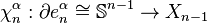 be the attaching map. Then consider the composition

where the first map identifies  with
with  via the characteristic map
  of , the object
  is an
is an  -cell of X, the third map
  is the quotient map that collapses
  to a point (thus wrapping into a sphere ), and the last map identifies
 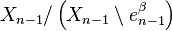 with via the characteristic map
  of .
of .
The boundary map

is then given by the formula
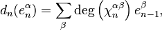
where  is the degree of
  and the sum is taken over all -cells of , considered as generators of
 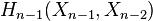 .
.
Example
The n-dimensional sphere Sn admits a CW structure with two cells, one 0-cell and one n-cell. Here the n-cell is attached by the constant mapping from  to 0-cell. Since the generators of the cellular homology groups
  can be identified with the k-cells of Sn, we have that
  for
for  and is otherwise trivial.
Hence for  , the resulting chain complex is

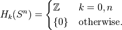
but then as all the boundary maps are either to or from trivial groups, they must all be zero, meaning that the cellular homology groups are equal to
When  , it is not very difficult to verify that the boundary map
  is zero, meaning the above formula holds for all positive .
As this example shows, computations done with cellular homology are often more efficient than those calculated by using singular homology alone.
Other Properties
One sees from the cellular-chain complex that the -skeleton determines all lower-dimensional homology modules:

for  .
.
An important consequence of this cellular perspective is that if a CW-complex has no cells in consecutive dimensions, then all of its homology modules are free. For example, the complex projective space  has a cell structure with one cell in each even dimension; it follows that for
  ,
,
and

Generalization
The Atiyah-Hirzebruch spectral sequence is the analogous method of computing the (co)homology of a CW-complex, for an arbitrary extraordinary (co)homology theory.
Euler Characteristic
For a cellular complex , let  be its
  -th skeleton, and
  be the number of -cells, i.e., the rank of the free module
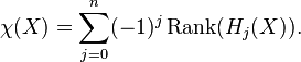
  . The Euler characteristic of is then defined by

The Euler characteristic is a homotopy invariant. In fact, in terms of the Betti numbers of ,
This can be justified as follows. Consider the long exact sequence of relative homology for the triple  :
:

Chasing exactness through the sequence gives

The same calculation applies to the triples  ,
,  , etc. By induction,

References
- A. Dold: Lectures on Algebraic Topology, Springer ISBN 3-540-58660-1.
- A. Hatcher: Algebraic Topology, Cambridge University Press ISBN 978-0-521-79540-1. A free electronic version is available on the author's homepage.