Propagator
| Quantum field theory |
|---|
 |
| History |
|
Incomplete theories |
|
Scientists
|
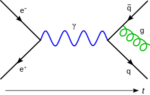
In quantum mechanics and quantum field theory, the propagator is a function that specifies the probability amplitude for a particle to travel from one place to another in a given time, or to travel with a certain energy and momentum. In Feynman diagrams, which serve to calculate the rate of collisions in quantum field theory, virtual particles contribute their propagator to the rate of the scattering event described by the respective diagram. These may also be viewed as the inverse of the wave operator appropriate to the particle, and are, therefore, often called (causal) Green's functions (called "causal" to distinguish it from the elliptic Laplacian Green's function).[1][2]
Non-relativistic propagators
In non-relativistic quantum mechanics, the propagator gives the probability amplitude for a particle to travel from one spatial point at one time to another spatial point at a later time. It is the Green's function (fundamental solution) for the Schrödinger equation. This means that, if a system has Hamiltonian H, then the appropriate propagator is a function

satisfying

where Hx denotes the Hamiltonian written in terms of the x coordinates, δ(x) denotes the Dirac delta-function, Θ(x) is the Heaviside step function and K(x, t ;x′, t′) is the kernel of the differential operator in question, often referred to as the propagator instead of G in this context, and henceforth in this article. This propagator can also be written as

where Û(t, t′) is the unitary time-evolution operator for the system taking states at time t to states at time t′.
The quantum mechanical propagator may also be found by using a path integral,
![{\displaystyle K(x,t;x',t')=\int \exp \left[{\frac {i}{\hbar }}\int _{t}^{t'}L({\dot {q}},q,t)\,dt\right]D[q(t)]}](../I/m/e955342647dcc12817f4053671bf1fce44f81416.svg)
where the boundary conditions of the path integral include q(t) = x, q(t′) = x′. Here L denotes the Lagrangian of the system. The paths that are summed over move only forwards in time.
In non-relativistic quantum mechanics, the propagator lets you find the state of a system given an initial state and a time interval. The new state is given by the equation

If K(x,t;x′,t′) only depends on the difference x − x′, this is a convolution of the initial state and the propagator. This kernel is the kernel of integral transform.
Basic examples: propagator of free particle and harmonic oscillator
For a time-translationally invariant system, the propagator only depends on the time difference t − t′, so it may be rewritten as

The propagator of a one-dimensional free particle, with the far-right expression obtained via saddle-point methods, is then

Similarly, the propagator of a one-dimensional quantum harmonic oscillator is the Mehler kernel,[3][4]

The latter may be obtained from the previous free particle result upon making use of van Kortryk's SU(2) Lie-group identity,


valid for operators and satisfying the Heisenberg relation .


![[{\mathsf {x}},{\mathsf {p}}]=i\hbar](../I/m/c34a6d2b647663cd1951f44edb2c69556a1c756a.svg)
For the N-dimensional case, the propagator can be simply obtained by the product

Relativistic propagators
In relativistic quantum mechanics and quantum field theory the propagators are Lorentz invariant. They give the amplitude for a particle to travel between two spacetime points.
Scalar propagator
In quantum field theory the theory of a free (non-interacting) scalar field is a useful and simple example which serves to illustrate the concepts needed for more complicated theories. It describes spin zero particles. There are a number of possible propagators for free scalar field theory. We now describe the most common ones.
Position space
The position space propagators are Green's functions for the Klein–Gordon equation. This means they are functions G(x, y) which satisfy

where:
- x, y are two points in Minkowski spacetime.
- is the d'Alembertian operator acting on the x coordinates.
- δ(x − y) is the Dirac delta-function.

(As typical in relativistic quantum field theory calculations, we use units where the speed of light, c, and Planck's reduced constant, ħ, are set to unity.)
We shall restrict attention to 4-dimensional Minkowski spacetime. We can perform a Fourier transform of the equation for the propagator, obtaining

This equation can be inverted in the sense of distributions noting that the equation xf(x)=1 has the solution, (see Sokhotski-Plemelj theorem)

with ε implying the limit to zero. Below, we discuss the right choice of the sign arising from causality requirements.
The solution is

where

is the 4-vector inner product.
The different choices for how to deform the integration contour in the above expression lead to different forms for the propagator. The choice of contour is usually phrased in terms of the integral.

The integrand then has two poles at

so different choices of how to avoid these lead to different propagators.
Causal propagators
Retarded propagator

A contour going clockwise over both poles gives the causal retarded propagator. This is zero if x and y are spacelike or if x ⁰< y ⁰ (i.e. if y is to the future of x).
This choice of contour is equivalent to calculating the limit,

Here

is the proper time from x to y and is a Bessel function of the first kind. The expression means y causally precedes x which, for Minkowski spacetime, means


- and


This expression can also be expressed in terms of the vacuum expectation value of the commutator of the free scalar field operator,
![{\displaystyle G_{\text{ret}}(x,y)=i\langle 0|\left[\Phi (x),\Phi (y)\right]|0\rangle \Theta (x^{0}-y^{0})}](../I/m/919d5e45fb1f438f28f4a192a3a521bd875ab1e0.svg)
where

is the Heaviside step function and
![\left[\Phi (x),\Phi (y)\right]:=\Phi (x)\Phi (y)-\Phi (y)\Phi (x)](../I/m/dd5c193518649d1efcc53776f9bf57231459b668.svg)
is the commutator.
Advanced propagator

A contour going anti-clockwise under both poles gives the causal advanced propagator. This is zero if x and y are spacelike or if x ⁰> y ⁰ (i.e. if y is to the past of x).
This choice of contour is equivalent to calculating the limit
![{\displaystyle {\begin{aligned}G_{\text{adv}}(x,y)&=\lim _{\varepsilon \to 0}{\frac {1}{(2\pi )^{4}}}\int d^{4}p\,{\frac {e^{-ip(x-y)}}{(p_{0}-i\varepsilon )^{2}-{\vec {p}}^{2}-m^{2}}}\\[6pt]&={\begin{cases}-{\frac {1}{2\pi }}\delta (\tau _{xy}^{2})+{\frac {mJ_{1}(m\tau _{xy})}{4\pi \tau _{xy}}}&x\prec y\\0&{\textrm {otherwise}}\end{cases}}\end{aligned}}}](../I/m/ac60e3ff5318752eeb209273f0d37002159c8ffc.svg)
This expression can also be expressed in terms of the vacuum expectation value of the commutator of the free scalar field. In this case,
![{\displaystyle G_{\text{adv}}(x,y)=-i\langle 0|\left[\Phi (x),\Phi (y)\right]|0\rangle \Theta (y^{0}-x^{0})~.}](../I/m/52c088b6e64f0a02c16f81454d3e5b1c71956360.svg)
Feynman propagator
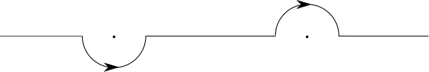
A contour going under the left pole and over the right pole gives the Feynman propagator.
This choice of contour is equivalent to calculating the limit (see Huang p. 30)

Here

where x and y are two points in Minkowski spacetime, and the dot in the exponent is a four-vector inner product. H1(2) is a Hankel function and K1 is a modified Bessel function.
This expression can be derived directly from the field theory as the vacuum expectation value of the time-ordered product of the free scalar field, that is, the product always taken such that the time ordering of the spacetime points is the same,
![{\displaystyle {\begin{aligned}G_{F}(x-y)&=-i\langle 0|T(\Phi (x)\Phi (y))|0\rangle \\[4pt]&=-i\left\langle 0|\left[\Theta (x^{0}-y^{0})\Phi (x)\Phi (y)+\Theta (y^{0}-x^{0})\Phi (y)\Phi (x)\right]|0\right\rangle .\end{aligned}}}](../I/m/464fd25d8ac399c3cdc9869a3ebb74e23bc6c607.svg)
This expression is Lorentz invariant, as long as the field operators commute with one another when the points x and y are separated by a spacelike interval.
The usual derivation is to insert a complete set of single-particle momentum states between the fields with Lorentz covariant normalization, then show that the Θ functions providing the causal time ordering may be obtained by a contour integral along the energy axis if the integrand is as above (hence the infinitesimal imaginary part, to move the pole off the real line).
The propagator may also be derived using the path integral formulation of quantum theory.
Momentum space propagator
The Fourier transform of the position space propagators can be thought of as propagators in momentum space. These take a much simpler form than the position space propagators.
They are often written with an explicit ε term although this is understood to be a reminder about which integration contour is appropriate (see above). This ε term is included to incorporate boundary conditions and causality (see below).
For a 4-momentum p the causal and Feynman propagators in momentum space are:


For purposes of Feynman diagram calculations it is usually convenient to write these with an additional overall factor of −i (conventions vary).
Faster than light?
The Feynman propagator has some properties that seem baffling at first. In particular, unlike the commutator, the propagator is nonzero outside of the light cone, though it falls off rapidly for spacelike intervals. Interpreted as an amplitude for particle motion, this translates to the virtual particle traveling faster than light. It is not immediately obvious how this can be reconciled with causality: can we use faster-than-light virtual particles to send faster-than-light messages?
The answer is no: while in classical mechanics the intervals along which particles and causal effects can travel are the same, this is no longer true in quantum field theory, where it is commutators that determine which operators can affect one another.
So what does the spacelike part of the propagator represent? In QFT the vacuum is an active participant, and particle numbers and field values are related by an uncertainty principle; field values are uncertain even for particle number zero. There is a nonzero probability amplitude to find a significant fluctuation in the vacuum value of the field Φ(x) if one measures it locally (or, to be more precise, if one measures an operator obtained by averaging the field over a small region). Furthermore, the dynamics of the fields tend to favor spatially correlated fluctuations to some extent. The nonzero time-ordered product for spacelike-separated fields then just measures the amplitude for a nonlocal correlation in these vacuum fluctuations, analogous to an EPR correlation. Indeed, the propagator is often called a two-point correlation function for the free field.
Since, by the postulates of quantum field theory, all observable operators commute with each other at spacelike separation, messages can no more be sent through these correlations than they can through any other EPR correlations; the correlations are in random variables.
In terms of virtual particles, the propagator at spacelike separation can be thought of as a means of calculating the amplitude for creating a virtual particle-antiparticle pair that eventually disappear into the vacuum, or for detecting a virtual pair emerging from the vacuum. In Feynman's language, such creation and annihilation processes are equivalent to a virtual particle wandering backward and forward through time, which can take it outside of the light cone. However, no causality violation is involved.
Explanation using limits
This can be made clearer by writing the propagator in the following form for a massless photon,

This is the usual definition but normalised by a factor of . Then the rule is that one only takes the limit at the end of a calculation.


One sees that
- if


and
- if


Hence this means a single photon will always stay on the light cone. It is also shown that the total probability for a photon at any time must be normalised by the reciprocal of the following factor:

We see that the parts outside the light cone usually are zero in the limit and only are important in Feynman diagrams.
Propagators in Feynman diagrams
The most common use of the propagator is in calculating probability amplitudes for particle interactions using Feynman diagrams. These calculations are usually carried out in momentum space. In general, the amplitude gets a factor of the propagator for every internal line, that is, every line that does not represent an incoming or outgoing particle in the initial or final state. It will also get a factor proportional to, and similar in form to, an interaction term in the theory's Lagrangian for every internal vertex where lines meet. These prescriptions are known as Feynman rules.
Internal lines correspond to virtual particles. Since the propagator does not vanish for combinations of energy and momentum disallowed by the classical equations of motion, we say that the virtual particles are allowed to be off shell. In fact, since the propagator is obtained by inverting the wave equation, in general it will have singularities on shell.
The energy carried by the particle in the propagator can even be negative. This can be interpreted simply as the case in which, instead of a particle going one way, its antiparticle is going the other way, and therefore carrying an opposing flow of positive energy. The propagator encompasses both possibilities. It does mean that one has to be careful about minus signs for the case of fermions, whose propagators are not even functions in the energy and momentum (see below).
Virtual particles conserve energy and momentum. However, since they can be off shell, wherever the diagram contains a closed loop, the energies and momenta of the virtual particles participating in the loop will be partly unconstrained, since a change in a quantity for one particle in the loop can be balanced by an equal and opposite change in another. Therefore, every loop in a Feynman diagram requires an integral over a continuum of possible energies and momenta. In general, these integrals of products of propagators can diverge, a situation that must be handled by the process of renormalization.
Other theories
Spin 1⁄2
If the particle possesses spin then its propagator is in general somewhat more complicated, as it will involve the particle's spin or polarization indices. The differential equation satisfied by the propagator for a spin 1⁄2 particle is given by[5]

where I4 is the unit matrix in four dimensions, and employing the Feynman slash notation. This is the Dirac equation for a delta function source in spacetime. Using the momentum representation,
![{\displaystyle S_{F}(x',x)=\int {\frac {d^{4}p}{(2\pi )^{4}}}\exp {\left[-ip\cdot (x'-x)\right]}{\tilde {S}}_{F}(p),}](../I/m/81a71c7f8b3f04f80e0b46f8ef96cc872982365b.svg)
the equation becomes
![{\displaystyle {\begin{aligned}&(i\not \nabla '-m)\int {\frac {d^{4}p}{(2\pi )^{4}}}{\tilde {S}}_{F}(p)\exp {\left[-ip\cdot (x'-x)\right]}\\[6pt]={}&\int {\frac {d^{4}p}{(2\pi )^{4}}}(\not p-m){\tilde {S}}_{F}(p)\exp {\left[-ip\cdot (x'-x)\right]}\\[6pt]={}&\int {\frac {d^{4}p}{(2\pi )^{4}}}I_{4}\exp {\left[-ip\cdot (x'-x)\right]}\\[6pt]={}&I_{4}\delta ^{4}(x'-x),\end{aligned}}}](../I/m/4770a7ba0dbc05aa4f9d98e0faa34cb1b94c9a51.svg)
where on the right hand side an integral representation of the four-dimensional delta function is used. Thus

By multiplying from the left with

(dropping unit matrices from the notation) and using properties of the gamma matrices,
![{\displaystyle {\begin{aligned}\not p\not p&={\frac {1}{2}}(\not p\not p+\not p\not p)\\[6pt]&={\frac {1}{2}}(\gamma _{\mu }p^{\mu }\gamma _{\nu }p^{\nu }+\gamma _{\nu }p^{\nu }\gamma _{\mu }p^{\mu })\\[6pt]&={\frac {1}{2}}(\gamma _{\mu }\gamma _{\nu }+\gamma _{\nu }\gamma _{\mu })p^{\mu }p^{\nu }\\[6pt]&=g_{\mu \nu }p^{\mu }p^{\nu }=p_{\mu }p^{\nu }=p^{2},\end{aligned}}}](../I/m/a79eb5ed856ba0ec99a68405ad96948e7e1a9972.svg)
the momentum-space propagator used in Feynman diagrams for a Dirac field representing the electron in quantum electrodynamics is found to have form

The iε downstairs is a prescription for how to handle the poles in the complex p0-plane. It automatically yields the Feynman contour of integration by shifting the poles appropriately. It is sometimes written

for short. It should be remembered that this expression is just shorthand notation for (γμpμ − m)−1. "One over matrix" is otherwise nonsensical. In position space one has

This is related to the Feynman propagator by

where .

Spin 1
The propagator for a gauge boson in a gauge theory depends on the choice of convention to fix the gauge. For the gauge used by Feynman and Stueckelberg, the propagator for a photon is

The propagator for a massive vector field can be derived from the Stueckelberg Lagrangian. The general form with gauge parameter λ reads

With this general form one obtains the propagator in unitary gauge for λ = 0, the propagator in Feynman or 't Hooft gauge for λ = 1 and in Landau or Lorenz gauge for λ = ∞. There are also other notations where the gauge parameter is the inverse of λ. The name of the propagator however refers to its final form and not necessarily to the value of the gauge parameter.
Unitary gauge:

Feynman ('t Hooft) gauge:

Landau (Lorenz) gauge:

Graviton propagator
The graviton propagator for Minkowski space in general relativity is

where is the transverse and traceless spin-2 projection operator and is a spin-0 scalar multiplet. The graviton propagator for (Anti) de Sitter space is


where is the Hubble constant. Note that upon taking the limit , the AdS propagator reduces to the Minkowski propagator.[6]


Related singular functions
The scalar propagators are Green's functions for the Klein–Gordon equation. There are related singular functions which are important in quantum field theory. We follow the notation in Bjorken and Drell.[7] See also Bogolyubov and Shirkov (Appendix A). These function are most simply defined in terms of the vacuum expectation value of products of field operators.
Solutions to the Klein–Gordon equation
Pauli–Jordan function
The commutator of two scalar field operators defines the Pauli–Jordan function by[7]

![\langle 0|\left[\Phi (x),\Phi (y)\right]|0\rangle =i\Delta (x-y)](../I/m/6c2f008f5cf78aa8d40e214026dc7c879490cf3a.svg)
with

This satisfies

and is zero if .

Positive and negative frequency parts (cut propagators)
We can define the positive and negative frequency parts of , sometimes called cut propagators, in a relativistically invariant way.
This allows us to define the positive frequency part:

and the negative frequency part:

These satisfy[7]

and

Auxiliary function
The anti-commutator of two scalar field operators defines function by


with

This satisfies

Green's functions for the Klein–Gordon equation
The retarded, advanced and Feynman propagators defined above are all Green's functions for the Klein–Gordon equation.
They are related to the singular functions by[7]


where

Notes
- ↑ The mathematics of PDEs and the wave equation, p 32., Michael P. Lamoureux, University of Calgary, Seismic Imaging Summer School, August 7–11, 2006, Calgary.
- ↑ Ch.: 9 Green’s functions, p 6., J Peacock, FOURIER ANALYSIS LECTURE COURSE: LECTURE 15.
- ↑ E. U. Condon, "Immersion of the Fourier transform in a continuous group of functional transformations", Proc. Natl. Acad. Sci. USA 23, (1937) 158–164. online
- ↑ Wolfgang Pauli, Wave Mechanics: Volume 5 of Pauli Lectures on Physics (Dover Books on Physics, 2000) ISBN 0486414620 , cf. Section 44.
- ↑ Greiner & Reinhardt 2008, Ch.2
- ↑ "Graviton and gauge boson propagators in AdSd+1" (PDF).
- 1 2 3 4 Bjorken and Drell, Appendix C
References
- Bjorken, J.; Drell, S. (1965). Relativistic Quantum Fields. New York: McGraw-Hill. ISBN 0-07-005494-0. (Appendix C.)
- Bogoliubov, N.; Shirkov, D. V. Introduction to the theory of quantized fields. Wiley-Interscience. ISBN 0-470-08613-0. (Especially pp. 136–156 and Appendix A)
- DeWitt-Morette, C.; DeWitt, B. (eds.). Relativity, Groups and Topology. Glasgow: Blackie and Son. ISBN 0-444-86858-5. (section Dynamical Theory of Groups & Fields, Especially pp. 615–624)
- Greiner, W.; Reinhardt, J. (2008). Quantum Electrodynamics (4th ed.). Springer Verlag. ISBN 9783540875604.
- Greiner, W.; Reinhardt, J. (1996). Field Quantization. Springer Verlag. ISBN 9783540591795.
- Griffiths, D. J. (1987). Introduction to Elementary Particles. New York: John Wiley & Sons. ISBN 0-471-60386-4.
- Griffiths, D. J. (2004). Introduction to Quantum Mechanics. Upper Saddle River: Prentice Hall. ISBN 0-131-11892-7.
- Halliwell, J.J.; Orwitz, M., Sum-over-histories origin of the composition laws of relativistic quantum mechanics and quantum cosmology, arXiv:gr-qc/9211004
 , Bibcode:1993PhRvD..48..748H, doi:10.1103/PhysRevD.48.748
 - Huang, Kerson (1998). Quantum Field Theory: From Operators to Path Integrals. New York: John Wiley & Sons. ISBN 0-471-14120-8.
- Itzykson, C.; Zuber, J-B. (1980). Quantum Field Theory. New York: McGraw-Hill. ISBN 0-07-032071-3.
- Pokorski, S. (1987). Gauge Field Theories. Cambridge: Cambridge University Press. ISBN 0-521-36846-4. (Has useful appendices of Feynman diagram rules, including propagators, in the back.)
- Schulman, L. S. (1981). Techniques & Applications of Path Integration. New York: John Wiley & Sons. ISBN 0-471-76450-7.