First-order hold

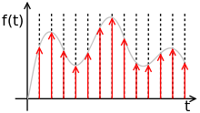
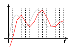
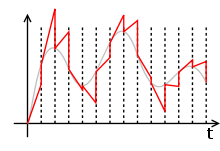
The first-order hold (FOH) is a mathematical model of the practical reconstruction of sampled signals that could be done by a conventional digital-to-analog converter (DAC) and an analog circuit called an integrator. For the FOH, the signal is reconstructed as a piecewise linear approximation to the original signal that was sampled. A mathematical model such as the FOH (or, more commonly, the zero-order hold) is necessary because, in the sampling and reconstruction theorem, a sequence of Dirac impulses, x_s(t), representing the discrete samples, x(nT), is low-pass filtered to recover the original signal that was sampled, x(t). However, outputting a sequence of Dirac impulses is impractical. Devices can be implemented, using a conventional DAC and some linear analog circuitry, to reconstruct the piecewise linear output for either the predictive or delayed FOH.

Even though this is not what is physically done, an identical output can be generated by applying the hypothetical sequence of Dirac impulses, x_s(t), to a linear, time-invariant system, otherwise known as a linear filter with such characteristics (which, for an LTI system, are fully described by the impulse response) so that each input impulse results in the correct piecewise linear function in the output.

Basic first-order hold

Ideally sampled signal x_s(t).

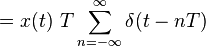
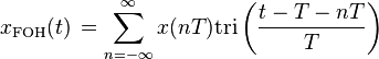
The first-order hold is the hypothetical filter or LTI system that converts the ideally sampled signal

$x_s(t)\,$	$= x(t) \ T \sum_{n=-\infty}^{\infty} \delta(t - nT) \$
	$= T \sum_{n=-\infty}^{\infty} x(nT) \delta(t - nT) \$

Piecewise linear signal x_FOH(t).

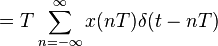
to the piecewise linear signal

$x_{\mathrm{FOH}}(t)\,= \sum_{n=-\infty}^{\infty} x(nT) \mathrm{tri} \left(\frac{t - nT}{T} \right) \$

Impulse response (non-causal) of first-order hold h_FOH(t).

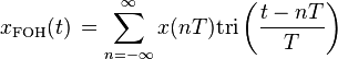
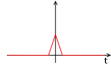
resulting in an effective impulse response of

$h_{\mathrm{FOH}}(t)\,= \frac{1}{T} \mathrm{tri} \left(\frac{t}{T} \right) = \begin{cases} \frac{1}{T} \left( 1 - \frac{|t|}{T} \right) & \mbox{if } |t| < T \\ 0 & \mbox{otherwise} \end{cases} \$

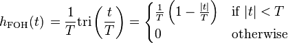
where $\mathrm{tri}(x) \$ is the triangular function.

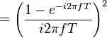
The effective frequency response is the continuous Fourier transform of the impulse response.

$H_{\mathrm{FOH}}(f)\,$	$= \mathcal{F} \{ h_{\mathrm{FOH}}(t) \} \$
	$= \left( \frac{e^{i \pi fT} - e^{-i \pi fT}}{i 2 \pi fT} \right)^2 \$
	$= \mathrm{sinc}^2(fT) \$

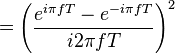
where $\mathrm{sinc}(x) = \frac{\sin(\pi x)}{\pi x} \$ is the normalized sinc function.

The Laplace transform transfer function of the FOH is found by substituting s = i 2 π f:

$H_{\mathrm{FOH}}(s)\,$	$= \mathcal{L} \{ h_{\mathrm{FOH}}(t) \} \$
	$= \left( \frac{e^{sT/2} - e^{-sT/2}}{sT} \right)^2 \$

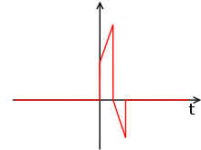
This is an acausal system in that the linear interpolation function moves toward the value of the next sample before such sample is applied to the hypothetical FOH filter. This acausality is also reflected in the impulse response of the FOH filter beginning to respond before impulse is applied.

Delayed first-order hold

Delayed piecewise linear signal x_FOH(t).

The delayed first-order hold, sometimes called causal first-order hold, is identical to the FOH above except that its output is delayed by one sample period resulting in a delayed piecewise linear output signal

$x_{\mathrm{FOH}}(t)\,= \sum_{n=-\infty}^{\infty} x(nT) \mathrm{tri} \left(\frac{t - T - nT}{T} \right) \$

Impulse response of causal first-order hold h_FOH(t).

resulting in an effective impulse response of

$h_{\mathrm{FOH}}(t)\,= \frac{1}{T} \mathrm{tri} \left(\frac{t-T}{T} \right) = \begin{cases} \frac{1}{T} \left( 1 - \frac{|t-T|}{T} \right) & \mbox{if } |t-T| < T \\ 0 & \mbox{otherwise} \end{cases} \$

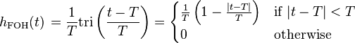
where $\mathrm{tri}(x) \$ is the triangular function.

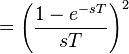
The effective frequency response is the continuous Fourier transform of the impulse response.

$H_{\mathrm{FOH}}(f)\,$	$= \mathcal{F} \{ h_{\mathrm{FOH}}(t) \} \$
	$= \left( \frac{1 - e^{-i 2\pi fT}}{i 2 \pi fT} \right)^2 \$
	$= e^{-i 2 \pi fT} \mathrm{sinc}^2(fT) \$

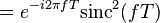
where $\mathrm{sinc}(x) \$ is the sinc function.

The Laplace transform transfer function of the delayed FOH is found by substituting s = i 2 π f:

$H_{\mathrm{FOH}}(s)\,$	$= \mathcal{L} \{ h_{\mathrm{FOH}}(t) \} \$
	$= \left( \frac{1 - e^{-sT}}{sT} \right)^2 \$

The delayed output makes this a causal system. The impulse response of the delayed FOH does not respond before the input impulse.

This kind of delayed piecewise linear reconstruction is physically realizable by implementing a digital filter of gain H(z) = 1 − z⁻¹, applying the output of that digital filter (which is simply x[n]−x[n−1]) to an ideal conventional digital-to-analog converter (that has an inherent zero-order hold as its model) and integrating (in continuous-time, H(s) = 1/(sT)) the DAC output.

Predictive first-order hold

Predictive FOH output signal x_FOH(t).

Lastly, the predictive first-order hold is quite different. This is a causal hypothetical LTI system or filter that converts the ideally sampled signal

$x_s(t)\,$	$= x(t) \ T \sum_{n=-\infty}^{\infty} \delta(t - nT) \$
	$= T \sum_{n=-\infty}^{\infty} x(nT) \delta(t - nT) \$

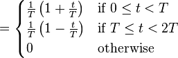
into a piecewise linear output such that the current sample and immediately previous sample are used to linearly extrapolate up to the next sampling instance. The output of such a filter would be

$x_{\mathrm{FOH}}(t)\,$	$= \sum_{n=-\infty}^{\infty} \left( x(nT) + \left( x(nT) - x((n-1)T) \right) \frac{t-nT}{T} \right) \mathrm{rect} \left(\frac{t - nT}{T} - \frac{1}{2} \right) \$
	$= \sum_{n=-\infty}^{\infty} x(nT) \left( \mathrm{rect} \left(\frac{t - nT}{T} - \frac{1}{2} \right) - \mathrm{rect} \left(\frac{t - nT}{T} - \frac{3}{2} \right) + \mathrm{tri} \left(\frac{t - nT}{T} - 1 \right) \right) \$

Impulse response of predictive first-order hold h_FOH(t).

resulting in an effective impulse response of

$h_{\mathrm{FOH}}(t)\,$	$= \frac{1}{T} \left( \mathrm{rect} \left(\frac{t}{T} - \frac{1}{2} \right) - \mathrm{rect} \left(\frac{t}{T} - \frac{3}{2} \right) + \mathrm{tri} \left(\frac{t}{T} -1 \right) \right) \$
	$= \begin{cases} \frac{1}{T} \left( 1 + \frac{t}{T} \right) & \mbox{if } 0 \le t < T \\ \frac{1}{T} \left( 1 - \frac{t}{T} \right) & \mbox{if } T \le t < 2T \\ 0 & \mbox{otherwise} \end{cases} \$

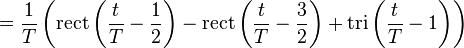
where $\mathrm{rect}(x) \$ is the rectangular function and $\mathrm{tri}(x) \$ is the triangular function.

The effective frequency response is the continuous Fourier transform of the impulse response.

$H_{\mathrm{FOH}}(f)\,$	$= \mathcal{F} \{ h_{\mathrm{FOH}}(t) \} \$
	$= (1 + i 2\pi fT) \left( \frac{1 - e^{-i 2\pi fT}}{i 2\pi fT} \right)^2 \$
	$= (1 + i 2\pi fT) e^{-i 2\pi fT} \mathrm{sinc}^2(fT)) \$

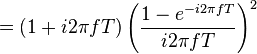
where $\mathrm{sinc}(x) \$ is the sinc function.

The Laplace transform transfer function of the predictive FOH is found by substituting s = i 2 π f:

$H_{\mathrm{FOH}}(s)\,$	$= \mathcal{L} \{ h_{\mathrm{FOH}}(t) \} \$
	$= (1 + sT) \left( \frac{1 - e^{-sT}}{sT} \right)^2 \$

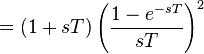
This a causal system. The impulse response of the predictive FOH does not respond before the input impulse.

This kind of piecewise linear reconstruction is physically realizable by implementing a digital filter of gain H(z) = 1 − z⁻¹, applying the output of that digital filter (which is simply x[n]−x[n−1]) to an ideal conventional digital-to-analog converter (that has an inherent zero-order hold as its model) and applying that DAC output to an analog filter with transfer function H(s) = (1+sT)/(sT).

See also

• Nyquist–Shannon sampling theorem
• Zero-order hold
• Bilinear interpolation

External links

• Zero order hold and first order hold based interpolation