Hierarchical clustering
| Machine learning and data mining |
|---|
 |
|
Machine learning venues
|
|
In data mining and statistics, hierarchical clustering (also called hierarchical cluster analysis or HCA) is a method of cluster analysis which seeks to build a hierarchy of clusters. Strategies for hierarchical clustering generally fall into two types:[1]
- Agglomerative: This is a "bottom up" approach: each observation starts in its own cluster, and pairs of clusters are merged as one moves up the hierarchy.
- Divisive: This is a "top down" approach: all observations start in one cluster, and splits are performed recursively as one moves down the hierarchy.
In general, the merges and splits are determined in a greedy manner. The results of hierarchical clustering are usually presented in a dendrogram.
In the general case, the complexity of agglomerative clustering is ,[1] which makes them too slow for large data sets. Divisive clustering with an exhaustive search is , which is even worse. However, for some special cases, optimal efficient agglomerative methods (of complexity ) are known: SLINK[2] for single-linkage and CLINK[3] for complete-linkage clustering.


Cluster dissimilarity
In order to decide which clusters should be combined (for agglomerative), or where a cluster should be split (for divisive), a measure of dissimilarity between sets of observations is required. In most methods of hierarchical clustering, this is achieved by use of an appropriate metric (a measure of distance between pairs of observations), and a linkage criterion which specifies the dissimilarity of sets as a function of the pairwise distances of observations in the sets.
Metric
The choice of an appropriate metric will influence the shape of the clusters, as some elements may be close to one another according to one distance and farther away according to another. For example, in a 2-dimensional space, the distance between the point (1,0) and the origin (0,0) is always 1 according to the usual norms, but the distance between the point (1,1) and the origin (0,0) can be 2 under Manhattan distance, under Euclidean distance, or 1 under maximum distance.

Some commonly used metrics for hierarchical clustering are:[4]
| Names | Formula |
|---|---|
| Euclidean distance | |
| Squared Euclidean distance | |
| Manhattan distance | |
| maximum distance | |
| Mahalanobis distance | where S is the Covariance matrix |


For text or other non-numeric data, metrics such as the Hamming distance or Levenshtein distance are often used.
A review of cluster analysis in health psychology research found that the most common distance measure in published studies in that research area is the Euclidean distance or the squared Euclidean distance.
Linkage criteria
The linkage criterion determines the distance between sets of observations as a function of the pairwise distances between observations.
Some commonly used linkage criteria between two sets of observations A and B are:[5][6]
| Names | Formula |
|---|---|
| Maximum or complete-linkage clustering | |
| Minimum or single-linkage clustering | |
| Mean or average linkage clustering, or UPGMA | |
| Centroid linkage clustering, or UPGMC | where and are the centroids of clusters s and t, respectively. |
| Minimum energy clustering |


where d is the chosen metric. Other linkage criteria include:
- The sum of all intra-cluster variance.
- The decrease in variance for the cluster being merged (Ward's criterion).[7]
- The probability that candidate clusters spawn from the same distribution function (V-linkage).
- The product of in-degree and out-degree on a k-nearest-neighbour graph (graph degree linkage).[8]
- The increment of some cluster descriptor (i.e., a quantity defined for measuring the quality of a cluster) after merging two clusters.[9][10][11]
Discussion
Hierarchical clustering has the distinct advantage that any valid measure of distance can be used. In fact, the observations themselves are not required: all that is used is a matrix of distances.
Agglomerative clustering example
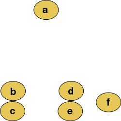
For example, suppose this data is to be clustered, and the Euclidean distance is the distance metric.
Cutting the tree at a given height will give a partitioning clustering at a selected precision. In this example, cutting after the second row of the dendrogram will yield clusters {a} {b c} {d e} {f}. Cutting after the third row will yield clusters {a} {b c} {d e f}, which is a coarser clustering, with a smaller number but larger clusters.
The hierarchical clustering dendrogram would be as such:
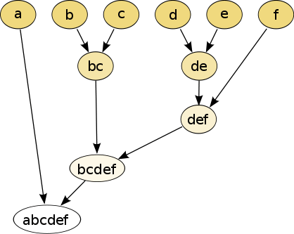
This method builds the hierarchy from the individual elements by progressively merging clusters. In our example, we have six elements {a} {b} {c} {d} {e} and {f}. The first step is to determine which elements to merge in a cluster. Usually, we want to take the two closest elements, according to the chosen distance.
Optionally, one can also construct a distance matrix at this stage, where the number in the i-th row j-th column is the distance between the i-th and j-th elements. Then, as clustering progresses, rows and columns are merged as the clusters are merged and the distances updated. This is a common way to implement this type of clustering, and has the benefit of caching distances between clusters. A simple agglomerative clustering algorithm is described in the single-linkage clustering page; it can easily be adapted to different types of linkage (see below).
Suppose we have merged the two closest elements b and c, we now have the following clusters {a}, {b, c}, {d}, {e} and {f}, and want to merge them further. To do that, we need to take the distance between {a} and {b c}, and therefore define the distance between two clusters. Usually the distance between two clusters and is one of the following:


- The maximum distance between elements of each cluster (also called complete-linkage clustering):

- The minimum distance between elements of each cluster (also called single-linkage clustering):

- The mean distance between elements of each cluster (also called average linkage clustering, used e.g. in UPGMA):

- The sum of all intra-cluster variance.
- The decrease in variance for the cluster being merged (Ward's method[7])
- The probability that candidate clusters spawn from the same distribution function (V-linkage).
Each agglomeration occurs at a greater distance between clusters than the previous agglomeration, and one can decide to stop clustering either when the clusters are too far apart to be merged (distance criterion) or when there is a sufficiently small number of clusters (number criterion).
Divisive clustering
The basic principle of divisive clustering was published as the DIANA (DIvisive ANAlysis Clustering) algorithm.[12] Initially, all data is in the same cluster, and the largest cluster is split until every object is separate. Because there exist ways of splitting each cluster, heuristics are needed. DIANA chooses the object with the maximum average dissimilarity and then moves all objects to this cluster that are more similar to the new cluster than to the remainder. An obvious alternate choice is k-means clustering with ,[13] but any other clustering algorithm can be used that always produces at least two clusters.

Software
Open source implementations

- Cluster 3.0 provides a Graphical User Interface to access to different clustering routines and is available for Windows, Mac OS X, Linux, Unix.
- ELKI includes multiple hierarchical clustering algorithms, various linkage strategies and also includes the efficient SLINK,[2] CLINK[3] and Anderberg algorithms, flexible cluster extraction from dendrograms and various other cluster analysis algorithms.
- Octave, the GNU analog to MATLAB implements hierarchical clustering in linkage function
- Orange, a free data mining software suite, module orngClustering for scripting in Python, or cluster analysis through visual programming.
- R has several functions for hierarchical clustering: see CRAN Task View: Cluster Analysis & Finite Mixture Models for more information.
- SCaViS computing environment in Java that implements this algorithm.
- scikit-learn implements a hierarchical clustering.
- Weka includes hierarchical cluster analysis.
Commercial
- MATLAB includes hierarchical cluster analysis.
- SAS includes hierarchical cluster analysis in PROC CLUSTER.[14]
- Mathematica includes a Hierarchical Clustering Package.
- NCSS (statistical software) includes hierarchical cluster analysis.
- SPSS includes hierarchical cluster analysis.
- Qlucore Omics Explorer includes hierarchical cluster analysis.
- Stata includes hierarchical cluster analysis.
See also
- Statistical distance
- Brown clustering
- Cladistics
- Cluster analysis
- Computational phylogenetics
- CURE data clustering algorithm
- Dendrogram
- Determining the number of clusters in a data set
- Hierarchical clustering of networks
- Nearest-neighbor chain algorithm
- Numerical taxonomy
- OPTICS algorithm
- Nearest neighbor search
- Locality-sensitive hashing
- Bounding volume hierarchy
- Binary space partitioning
References
- 1 2 Rokach, Lior, and Oded Maimon. "Clustering methods." Data mining and knowledge discovery handbook. Springer US, 2005. 321-352.
- 1 2 R. Sibson (1973). "SLINK: an optimally efficient algorithm for the single-link cluster method" (PDF). The Computer Journal. British Computer Society. 16 (1): 30–34. doi:10.1093/comjnl/16.1.30.
- 1 2 D. Defays (1977). "An efficient algorithm for a complete link method". The Computer Journal. British Computer Society. 20 (4): 364–366. doi:10.1093/comjnl/20.4.364.
- ↑ "The DISTANCE Procedure: Proximity Measures". SAS/STAT 9.2 Users Guide. SAS Institute. Retrieved 2009-04-26.
- ↑ "The CLUSTER Procedure: Clustering Methods". SAS/STAT 9.2 Users Guide. SAS Institute. Retrieved 2009-04-26.
- ↑ Székely, G. J. and Rizzo, M. L. (2005) Hierarchical clustering via Joint Between-Within Distances: Extending Ward's Minimum Variance Method, Journal of Classification 22, 151-183.
- 1 2 Ward, Joe H. (1963). "Hierarchical Grouping to Optimize an Objective Function". Journal of the American Statistical Association. 58 (301): 236–244. doi:10.2307/2282967. JSTOR 2282967. MR 0148188.
- ↑ Zhang, et al. "Graph degree linkage: Agglomerative clustering on a directed graph." 12th European Conference on Computer Vision, Florence, Italy, October 7–13, 2012. http://arxiv.org/abs/1208.5092
- ↑ Zhang, et al. "Agglomerative clustering via maximum incremental path integral." Pattern Recognition (2013).
- ↑ Zhao, and Tang. "Cyclizing clusters via zeta function of a graph."Advances in Neural Information Processing Systems. 2008.
- ↑ Ma, et al. "Segmentation of multivariate mixed data via lossy data coding and compression." IEEE Transactions on Pattern Analysis and Machine Intelligence, 29(9) (2007): 1546-1562.
- ↑ Kaufman, L., & Roussew, P. J. (1990). Finding Groups in Data - An Introduction to Cluster Analysis. A Wiley-Science Publication John Wiley & Sons.
- ↑ Steinbach, M., Karypis, G., & Kumar, V. (2000, August). A comparison of document clustering techniques. In KDD workshop on text mining (Vol. 400, No. 1, pp. 525-526).
- ↑ https://support.sas.com/documentation/cdl/en/statug/63033/HTML/default/viewer.htm#cluster_toc.htm
Further reading
- Kaufman, L.; Rousseeuw, P.J. (1990). Finding Groups in Data: An Introduction to Cluster Analysis (1 ed.). New York: John Wiley. ISBN 0-471-87876-6.
- Hastie, Trevor; Tibshirani, Robert; Friedman, Jerome (2009). "14.3.12 Hierarchical clustering". The Elements of Statistical Learning (PDF) (2nd ed.). New York: Springer. pp. 520–528. ISBN 0-387-84857-6. Retrieved 2009-10-20.