Perceptron
| Machine learning and data mining |
|---|
 |
|
Machine learning venues
|
|
In machine learning, the perceptron is an algorithm for supervised learning of binary classifiers (functions that can decide whether an input, represented by a vector of numbers, belongs to some specific class or not).[1] It is a type of linear classifier, i.e. a classification algorithm that makes its predictions based on a linear predictor function combining a set of weights with the feature vector. The algorithm allows for online learning, in that it processes elements in the training set one at a time.
The perceptron algorithm dates back to the late 1950s; its first implementation, in custom hardware, was one of the first artificial neural networks to be produced.
History
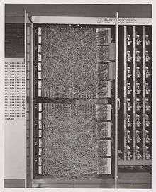
The perceptron algorithm was invented in 1957 at the Cornell Aeronautical Laboratory by Frank Rosenblatt,[3] funded by the United States Office of Naval Research.[4] The perceptron was intended to be a machine, rather than a program, and while its first implementation was in software for the IBM 704, it was subsequently implemented in custom-built hardware as the "Mark 1 perceptron". This machine was designed for image recognition: it had an array of 400 photocells, randomly connected to the "neurons". Weights were encoded in potentiometers, and weight updates during learning were performed by electric motors.[2]:193
In a 1958 press conference organized by the US Navy, Rosenblatt made statements about the perceptron that caused a heated controversy among the fledgling AI community; based on Rosenblatt's statements, The New York Times reported the perceptron to be "the embryo of an electronic computer that [the Navy] expects will be able to walk, talk, see, write, reproduce itself and be conscious of its existence."[4]
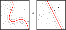
Although the perceptron initially seemed promising, it was quickly proved that perceptrons could not be trained to recognise many classes of patterns. This caused the field of neural network research to stagnate for many years, before it was recognised that a feedforward neural network with two or more layers (also called a multilayer perceptron) had far greater processing power than perceptrons with one layer (also called a single layer perceptron). Single layer perceptrons are only capable of learning linearly separable patterns; in 1969 a famous book entitled Perceptrons by Marvin Minsky and Seymour Papert showed that it was impossible for these classes of network to learn an XOR function. It is often believed that they also conjectured (incorrectly) that a similar result would hold for a multi-layer perceptron network. However, this is not true, as both Minsky and Papert already knew that multi-layer perceptrons were capable of producing an XOR function. (See the page on Perceptrons (book) for more information.) Three years later Stephen Grossberg published a series of papers introducing networks capable of modelling differential, contrast-enhancing and XOR functions. (The papers were published in 1972 and 1973, see e.g.:Grossberg (1973). "Contour enhancement, short-term memory, and constancies in reverberating neural networks" (PDF). Studies in Applied Mathematics. 52: 213–257.). Nevertheless, the often-miscited Minsky/Papert text caused a significant decline in interest and funding of neural network research. It took ten more years until neural network research experienced a resurgence in the 1980s. This text was reprinted in 1987 as "Perceptrons - Expanded Edition" where some errors in the original text are shown and corrected.
The kernel perceptron algorithm was already introduced in 1964 by Aizerman et al.[5] Margin bounds guarantees were given for the Perceptron algorithm in the general non-separable case first by Freund and Schapire (1998),[1] and more recently by Mohri and Rostamizadeh (2013) who extend previous results and give new L1 bounds.[6]
Definition
In the modern sense, the perceptron is an algorithm for learning a binary classifier: a function that maps its input (a real-valued vector) to an output value (a single binary value):


where w is a vector of real-valued weights, is the dot product , where m is the number of inputs to the perceptron and b is the bias. The bias shifts the decision boundary away from the origin and does not depend on any input value.


The value of (0 or 1) is used to classify x as either a positive or a negative instance, in the case of a binary classification problem. If is negative, then the weighted combination of inputs must produce a positive value greater than in order to push the classifier neuron over the 0 threshold. Spatially, the bias alters the position (though not the orientation) of the decision boundary. The perceptron learning algorithm does not terminate if the learning set is not linearly separable. If the vectors are not linearly separable learning will never reach a point where all vectors are classified properly. The most famous example of the perceptron's inability to solve problems with linearly nonseparable vectors is the Boolean exclusive-or problem. The solution spaces of decision boundaries for all binary functions and learning behaviors are studied in the reference.[7]


In the context of neural networks, a perceptron is an artificial neuron using the Heaviside step function as the activation function. The perceptron algorithm is also termed the single-layer perceptron, to distinguish it from a multilayer perceptron, which is a misnomer for a more complicated neural network. As a linear classifier, the single-layer perceptron is the simplest feedforward neural network.
Learning algorithm
Below is an example of a learning algorithm for a (single-layer) perceptron. For multilayer perceptrons, where a hidden layer exists, more sophisticated algorithms such as backpropagation must be used. Alternatively, methods such as the delta rule can be used if the function is non-linear and differentiable, although the one below will work as well.
When multiple perceptrons are combined in an artificial neural network, each output neuron operates independently of all the others; thus, learning each output can be considered in isolation.
Definitions
We first define some variables:
- denotes the output from the perceptron for an input vector .
- is the training set of samples, where:
- is the -dimensional input vector.
- is the desired output value of the perceptron for that input.


We show the values of the features as follows:
- is the value of the th feature of the th training input vector.
- .


To represent the weights:
- is the th value in the weight vector, to be multiplied by the value of the th input feature.
- Because , the is effectively a learned bias that we use instead of the bias constant .


To show the time-dependence of , we use:

- is the weight at time .


Unlike other linear classification algorithms such as logistic regression, there is no need for a learning rate in the perceptron algorithm. This is because multiplying the update by any constant simply rescales the weights but never changes the sign of the prediction.[8]

Steps
- Initialize the weights and the threshold. Weights may be initialized to 0 or to a small random value. In the example below, we use 0.
- For each example j in our training set D, perform the following steps over the input and desired output :
- Calculate the actual output:
- Update the weights:
- , for all features .
- Calculate the actual output:
- For offline learning, the step 2 may be repeated until the iteration error is less than a user-specified error threshold , or a predetermined number of iterations have been completed.

![{\displaystyle {\begin{aligned}y_{j}(t)&=f[\mathbf {w} (t)\cdot \mathbf {x} _{j}]\\&=f[w_{0}(t)x_{j,0}+w_{1}(t)x_{j,1}+w_{2}(t)x_{j,2}+\dotsb +w_{n}(t)x_{j,n}]\end{aligned}}}](../I/m/8e2650d5fbcec4f1b38ada11b50a95014aefbd6b.svg)


The algorithm updates the weights after steps 2a and 2b. These weights are immediately applied to a pair in the training set, and subsequently updated, rather than waiting until all pairs in the training set have undergone these steps.
Convergence
The perceptron is a linear classifier, therefore it will never get to the state with all the input vectors classified correctly if the training set D is not linearly separable, i.e. if the positive examples can not be separated from the negative examples by a hyperplane. In this case, no "approximate" solution will be gradually approached under the standard learning algorithm, but instead learning will fail completely. Hence, if linear separability of the training set is not known a priori, one of the training variants below should be used.
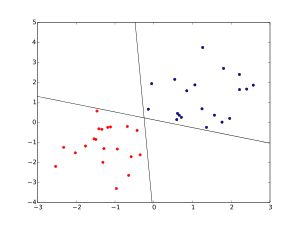
But if the training set is linearly separable, then the perceptron is guaranteed to converge, and there is an upper bound on the number of times the perceptron will adjust its weights during the training.
Suppose that the input vectors from the two classes can be separated by a hyperplane with a margin , i.e. there exists a weight vector , and a bias term b such that for all and for all . And also let R denote the maximum norm of an input vector. Novikoff (1962) proved that in this case the perceptron algorithm converges after making updates. The idea of the proof is that the weight vector is always adjusted by a bounded amount in a direction with which it has a negative dot product, and thus can be bounded above by O(√t) where t is the number of changes to the weight vector. But it can also be bounded below by O(t) because if there exists an (unknown) satisfactory weight vector, then every change makes progress in this (unknown) direction by a positive amount that depends only on the input vector.


While the perceptron algorithm is guaranteed to converge on some solution in the case of a linearly separable training set, it may still pick any solution and problems may admit many solutions of varying quality.[9] The perceptron of optimal stability, nowadays better known as the linear support vector machine, was designed to solve this problem.
Variants
The pocket algorithm with ratchet (Gallant, 1990) solves the stability problem of perceptron learning by keeping the best solution seen so far "in its pocket". The pocket algorithm then returns the solution in the pocket, rather than the last solution. It can be used also for non-separable data sets, where the aim is to find a perceptron with a small number of misclassifications. However, these solutions appear purely stochastically and hence the pocket algorithm neither approaches them gradually in the course of learning, nor are they guaranteed to show up within a given number of learning steps.
The Maxover algorithm (Wendemuth, 1995)[10] is "robust" in the sense that it will converge regardless of (prior) knowledge of linear separability of the data set. In the linear separable case, it will solve the training problem – if desired, even with optimal stability (maximum margin between the classes). For non-separable data sets, it will return a solution with a small number of misclassifications. In all cases, the algorithm gradually approaches the solution in the course of learning, without memorizing previous states and without stochastic jumps. Convergence is to global optimality for separable data sets and to local optimality for non-separable data sets.
In separable problems, perceptron training can also aim at finding the largest separating margin between the classes. The so-called perceptron of optimal stability can be determined by means of iterative training and optimization schemes, such as the Min-Over algorithm (Krauth and Mezard, 1987)[11] or the AdaTron (Anlauf and Biehl, 1989)) .[12] AdaTron uses the fact that the corresponding quadratic optimization problem is convex. The perceptron of optimal stability, together with the kernel trick, are the conceptual foundations of the support vector machine.
The -perceptron further used a pre-processing layer of fixed random weights, with thresholded output units. This enabled the perceptron to classify analogue patterns, by projecting them into a binary space. In fact, for a projection space of sufficiently high dimension, patterns can become linearly separable.

Another way to solve nonlinear problems without using multiple layers is to use higher order networks (sigma-pi unit). In this type of network, each element in the input vector is extended with each pairwise combination of multiplied inputs (second order). This can be extended to an n-order network.
It should be kept in mind, however, that the best classifier is not necessarily that which classifies all the training data perfectly. Indeed, if we had the prior constraint that the data come from equi-variant Gaussian distributions, the linear separation in the input space is optimal, and the nonlinear solution is overfitted.
Other linear classification algorithms include Winnow, support vector machine and logistic regression.
Multiclass perceptron
Like most other techniques for training linear classifiers, the perceptron generalizes naturally to multiclass classification. Here, the input and the output are drawn from arbitrary sets. A feature representation function maps each possible input/output pair to a finite-dimensional real-valued feature vector. As before, the feature vector is multiplied by a weight vector , but now the resulting score is used to choose among many possible outputs:


≈ Learning again iterates over the examples, predicting an output for each, leaving the weights unchanged when the predicted output matches the target, and changing them when it does not. The update becomes:

This multiclass feedback formulation reduces to the original perceptron when is a real-valued vector, is chosen from , and .


For certain problems, input/output representations and features can be chosen so that can be found efficiently even though is chosen from a very large or even infinite set.

In recent years, perceptron training has become popular in the field of natural language processing for such tasks as part-of-speech tagging and syntactic parsing (Collins, 2002).
References
- 1 2 Freund, Y.; Schapire, R. E. (1999). "Large margin classification using the perceptron algorithm" (PDF). Machine Learning. 37 (3): 277–296. doi:10.1023/A:1007662407062.
- 1 2 Bishop, Christopher M. (2006). Pattern Recognition and Machine Learning. Springer.
- ↑ Rosenblatt, Frank (1957), The Perceptron--a perceiving and recognizing automaton. Report 85-460-1, Cornell Aeronautical Laboratory.
- 1 2 Mikel Olazaran (1996). "A Sociological Study of the Official History of the Perceptrons Controversy". Social Studies of Science. 26 (3): 611–659. doi:10.1177/030631296026003005. JSTOR 285702.
- ↑ Aizerman, M. A.; Braverman, E. M.; Rozonoer, L. I. (1964). "Theoretical foundations of the potential function method in pattern recognition learning". Automation and Remote Control. 25: 821–837.
- ↑ Mohri, Mehryar and Rostamizadeh, Afshin (2013). Perceptron Mistake Bounds arXiv:1305.0208, 2013.
- ↑ Liou, D.-R.; Liou, J.-W.; Liou, C.-Y. (2013). Learning Behaviors of Perceptron. iConcept Press. ISBN 978-1-477554-73-9.
- ↑ https://www.willamette.edu/~gorr/classes/cs449/Classification/perceptron.html
- ↑ Bishop, Christopher M. "Chapter 4. Linear Models for Classification". Pattern Recognition and Machine Learning. Springer Science+Business Media, LLC. p. 194. ISBN 978-0387-31073-2.
- ↑ A. Wendemuth. Learning the Unlearnable. J. of Physics A: Math. Gen. 28: 5423-5436 (1995)
- ↑ W. Krauth and M. Mezard. Learning algorithms with optimal stability in neural networks. J. of Physics A: Math. Gen. 20: L745-L752 (1987)
- ↑ J.K. Anlauf and M. Biehl. The AdaTron: an Adaptive Perceptron algorithm. Europhysics Letters 10: 687-692 (1989)
- Aizerman, M. A. and Braverman, E. M. and Lev I. Rozonoer. Theoretical foundations of the potential function method in pattern recognition learning. Automation and Remote Control, 25:821–837, 1964.
- Rosenblatt, Frank (1958), The Perceptron: A Probabilistic Model for Information Storage and Organization in the Brain, Cornell Aeronautical Laboratory, Psychological Review, v65, No. 6, pp. 386–408. doi:10.1037/h0042519.
- Rosenblatt, Frank (1962), Principles of Neurodynamics. Washington, DC:Spartan Books.
- Minsky M. L. and Papert S. A. 1969. Perceptrons. Cambridge, MA: MIT Press.
- Gallant, S. I. (1990). Perceptron-based learning algorithms. IEEE Transactions on Neural Networks, vol. 1, no. 2, pp. 179–191.
- Mohri, Mehryar and Rostamizadeh, Afshin (2013). Perceptron Mistake Bounds arXiv:1305.0208, 2013.
- Novikoff, A. B. (1962). On convergence proofs on perceptrons. Symposium on the Mathematical Theory of Automata, 12, 615-622. Polytechnic Institute of Brooklyn.
- Widrow, B., Lehr, M.A., "30 years of Adaptive Neural Networks: Perceptron, Madaline, and Backpropagation," Proc. IEEE, vol 78, no 9, pp. 1415–1442, (1990).
- Collins, M. 2002. Discriminative training methods for hidden Markov models: Theory and experiments with the perceptron algorithm in Proceedings of the Conference on Empirical Methods in Natural Language Processing (EMNLP '02).
- Yin, Hongfeng (1996), Perceptron-Based Algorithms and Analysis, Spectrum Library, Concordia University, Canada
External links
- A Perceptron implemented in MATLAB to learn binary NAND function
- Chapter 3 Weighted networks - the perceptron and chapter 4 Perceptron learning of Neural Networks - A Systematic Introduction by Raúl Rojas (ISBN 978-3-540-60505-8)
- History of perceptrons
- Mathematics of perceptrons
- Explanation and Java implementation example