Linear complex structure

In mathematics, a complex structure on a real vector space V is an automorphism of V that squares to the minus identity, −I. Such a structure on V allows one to define multiplication by complex scalars in a canonical fashion so as to regard V as a complex vector space.

Every complex vector space can be equipped with a compatible complex structure, however, there is in general no canonical such structure. Complex structures have applications in representation theory as well as in complex geometry where they play an essential role in the definition of almost complex manifolds, by contrast to complex manifolds. The term "complex structure" often refers to this structure on manifolds; when it refers instead to a structure on vector spaces, it may be called a "linear complex structure".

Definition and properties

A complex structure on a real vector space V is a real linear transformation

J :V \rightarrow V

such that

J^2 = -\rm{Id}_V.

Here $J 2$ means $J$ composed with itself and $Id V$ is the identity map on $V$ . That is, the effect of applying $J$ twice is the same as multiplication by $- 1$ . This is reminiscent of multiplication by the imaginary unit, $i$ . A complex structure allows one to endow $V$ with the structure of a complex vector space. Complex scalar multiplication can be defined by

(x + iy)v = xv + yJ(v)

for all real numbers $x, y$ and all vectors $v$ in $V$ . One can check that this does, in fact, give $V$ the structure of a complex vector space which we denote $V J$ .

Going in the other direction, if one starts with a complex vector space $W$ then one can define a complex structure on the underlying real space by defining $Jw = iw$ for all $w \in W$ .

More formally, a linear complex structure on a real vector space is an algebra representation of the complex numbers $C$ , thought of as an associative algebra over the real numbers. This algebra is realized concretely as

\mathbf{C} = \mathbf{R}[x]/(x^2+1),

which corresponds to $i 2 = -1$ . Then a representation of $C$ is a real vector space $V$ , together with an action of $C$ on $V$ (a map $C \to End(V)$ ). Concretely, this is just an action of $i$ , as this generates the algebra, and the operator representing $i$ (the image of $i$ in $End(V)$ ) is exactly $J$ .

If $V J$ has complex dimension $n$ then $V$ must have real dimension $2 n$ . That is, a finite-dimensional space $V$ admits a complex structure only if it is even-dimensional. It is not hard to see that every even-dimensional vector space admits a complex structure. One can define $J$ on pairs $e, f$ of basis vectors by $Je = f$ and $Jf = - e$ and then extend by linearity to all of $V$ . If $(v 1, \dots, v n)$ is a basis for the complex vector space $V J$ then $(v 1, Jv 1, \dots, v n, Jv n)$ is a basis for the underlying real space $V$ .

A real linear transformation $A : V \to V$ is a complex linear transformation of the corresponding complex space $V J$ if and only if $A$ commutes with $J$ , i.e. if and only if

AJ = JA.

Likewise, a real subspace $U$ of $V$ is a complex subspace of $V J$ if and only if $J$ preserves $U$ , i.e. if and only if

JU = U.

Examples

Cⁿ

The fundamental example of a linear complex structure is the structure on R²ⁿ coming from the complex structure on Cⁿ. That is, the complex n-dimensional space Cⁿ is also a real 2n-dimensional space – using the same vector addition and real scalar multiplication – while multiplication by the complex number i is not only a complex linear transform of the space, thought of as a complex vector space, but also a real linear transform of the space, thought of as a real vector space. Concretely, this is because scalar multiplication by i commutes with scalar multiplication by real numbers $\qquad i (\lambda v) = (i \lambda) v = (\lambda i) v = \lambda (i v)\qquad$ – and distributes across vector addition. As a complex n×n matrix, this is simply the scalar matrix with i on the diagonal. The corresponding real 2n×2n matrix is denoted J.

Given a basis $\left\{e_1, e_2, \dots, e_n \right\}$ for the complex space, this set, together with these vectors multiplied by i, namely $\left\{ie_1, ie_2, \dots, ie_n\right\},$ form a basis for the real space. There are two natural ways to order this basis, corresponding abstractly to whether one writes the tensor product as $\mathbf{C}^n = \mathbf{R}^n \otimes_{\mathbf{R}} \mathbf{C}$ or instead as $\mathbf{C}^n = \mathbf{C} \otimes_{\mathbf{R}} \mathbf{R}^n.$

If one orders the basis as $\left\{e_1, ie_1, e_2, ie_2, \dots, e_n, ie_n\right\},$ then the matrix for J takes the block diagonal form (subscripts added to indicate dimension):

J_{2n} = \begin{bmatrix} 0 & -1 \\ 1 & 0 \\ & & 0 & -1 \\ & & 1 & 0 \\ & & & & \ddots \\ & & & & & \ddots \\ & & & & & & 0 & -1 \\ & & & & & & 1 & 0 \end{bmatrix} = \begin{bmatrix} J_2 \\ & J_2 \\ & & \ddots \\ & & & J_2 \end{bmatrix}.

This ordering has the advantage that it respects direct sums of complex vector spaces, meaning here that the basis for $\mathbf{C}^m \oplus \mathbf{C}^n$ is the same as that for $\mathbf{C}^{m+n}.$

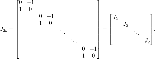
On the other hand, if one orders the basis as $\left\{e_1,e_2,\dots,e_n, ie_1, ie_2, \dots, ie_n\right\},$ then the matrix for J is block-antidiagonal:

J_{2n} = \begin{bmatrix}0 & -I_n \\ I_n & 0\end{bmatrix}.

This ordering is more natural if one thinks of the real space as a direct sum of real spaces, as discussed below.

The data of the real vector space and the J matrix is exactly the same as the data of the complex vector space, as the J matrix allows one to define complex multiplication. At the level of Lie algebras and Lie groups, this corresponds to the inclusion of gl(n,C) in gl(2n,R) (Lie algebras – matrices, not necessarily invertible) and GL(n,C) in GL(2n,R):

gl(n,C) < gl(2n,R) and GL(n,C) < GL(2n,R).

The inclusion corresponds to forgetting the complex structure (and keeping only the real), while the subgroup GL(n,C) can be characterized (given in equations) as the matrices that commute with J:

GL(n,C) =

\left\{ A \in GL(2n,\mathbf{R}) \mid AJ = JA \right\}.

The corresponding statement about Lie algebras is that the subalgebra gl(n,C) of complex matrices are those whose Lie bracket with J vanishes, meaning $[J,A] = 0;$ in other words, as the kernel of the map of bracketing with J, $[J,-].$

Note that the defining equations for these statements are the same, as AJ = JA is the same as 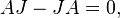$AJ - JA = 0,$ which is the same as $[A,J] = 0,$ though the meaning of the Lie bracket vanishing is less immediate geometrically than the meaning of commuting.

Direct sum

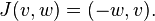
If V is any real vector space there is a canonical complex structure on the direct sum V ⊕ V given by

J(v,w) = (-w,v).\,

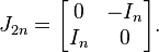
The block matrix form of J is

J = \begin{bmatrix}0 & -I_V \\ I_V & 0\end{bmatrix}

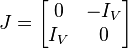
where $I_V$ is the identity map on V. This corresponds to the complex structure on the tensor product $\mathbf{C} \otimes_{\mathbf{R}} V.$

Compatibility with other structures

If $B$ is a bilinear form on $V$ then we say that $J$ preserves $B$ if

B(Ju, Jv) = B(u, v)

for all $u, v \in V$ . An equivalent characterization is that $J$ is skew-adjoint with respect to $B$ :

B(Ju, v) = -B(u, Jv)

If $g$ is an inner product on $V$ then $J$ preserves $g$ if and only if $J$ is an orthogonal transformation. Likewise, $J$ preserves a nondegenerate, skew-symmetric form $ω$ if and only if $J$ is a symplectic transformation (that is, if $ω(Ju, Jv) = ω(u, v))$ . For symplectic forms $ω$ there is usually an added restriction for compatibility between $J$ and $ω$ , namely

\omega(u, Ju) > 0

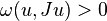
for all $u$ in $V$ . If this condition is satisfied then $J$ is said to tame $ω$ .

Given a symplectic form $ω$ and a linear complex structure $J$ , one may define an associated symmetric bilinear form $g J$ on $V J$

g_J(u, v) = \omega(u, Jv)

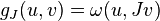Because a symplectic form is nondegenerate, so is the associated bilinear form. Moreover, the associated form is preserved by $J$ if and only if the symplectic form is, and if $ω$ is tamed by $J$ then the associated form is positive definite. Thus in this case the associated form is a Hermitian form and $V J$ is an inner product space.

Relation to complexifications

Given any real vector space V we may define its complexification by extension of scalars:

V^{\mathbb C}=V\otimes_{\mathbb{R}}\mathbb{C}.

This is a complex vector space whose complex dimension is equal to the real dimension of V. It has a canonical complex conjugation defined by

\overline{v\otimes z} = v\otimes\bar z

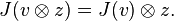
If J is a complex structure on V, we may extend J by linearity to V^C:

J(v\otimes z) = J(v)\otimes z.

Since C is algebraically closed, J is guaranteed to have eigenvalues which satisfy λ² = −1, namely λ = ±i. Thus we may write

V^{\mathbb C}= V^{+}\oplus V^{-}

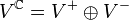
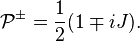
where V⁺ and V⁻ are the eigenspaces of +i and −i, respectively. Complex conjugation interchanges V⁺ and V⁻. The projection maps onto the V^± eigenspaces are given by

\mathcal P^{\pm} = {1\over 2}(1\mp iJ).

So that

V^{\pm} = \{v\otimes 1 \mp Jv\otimes i: v \in V\}.

There is a natural complex linear isomorphism between V_J and V⁺, so these vector spaces can be considered the same, while V⁻ may be regarded as the complex conjugate of V_J.

Note that if V_J has complex dimension n then both V⁺ and V⁻ have complex dimension n while V^C has complex dimension 2n.

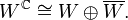
Abstractly, if one starts with a complex vector space W and takes the complexification of the underlying real space, one obtains a space isomorphic to the direct sum of W and its conjugate:

W^{\mathbb C} \cong W\oplus \overline{W}.

Extension to related vector spaces

Let V be a real vector space with a complex structure J. The dual space V* has a natural complex structure J* given by the dual (or transpose) of J. The complexification of the dual space (V*)^C therefore has a natural decomposition

(V^*)^\mathbb{C} = (V^*)^{+}\oplus (V^*)^-

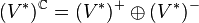
into the ±i eigenspaces of J*. Under the natural identification of (V*)^C with (V^C)* one can characterize (V*)⁺ as those complex linear functionals which vanish on V⁻. Likewise (V*)⁻ consists of those complex linear functionals which vanish on V⁺.

The (complex) tensor, symmetric, and exterior algebras over V^C also admit decompositions. The exterior algebra is perhaps the most important application of this decomposition. In general, if a vector space U admits a decomposition U = S ⊕ T then the exterior powers of U can be decomposed as follows:

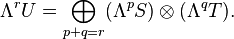
\Lambda^r U = \bigoplus_{p+q=r}(\Lambda^p S)\otimes(\Lambda^q T).

A complex structure J on V therefore induces a decomposition

\Lambda^r\,V^\mathbb{C} = \bigoplus_{p+q=r} \Lambda^{p,q}\,V_J

where

\Lambda^{p,q}\,V_J\;\stackrel{\mathrm{def}}{=}\, (\Lambda^p\,V^+)\otimes(\Lambda^q\,V^-).

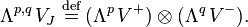
All exterior powers are taken over the complex numbers. So if V_J has complex dimension n (real dimension 2n) then

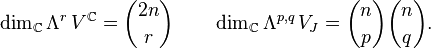
\dim_{\mathbb C}\Lambda^{r}\,V^{\mathbb C} = {2n\choose r}\qquad \dim_{\mathbb C}\Lambda^{p,q}\,V_J = {n \choose p}{n \choose q}.

The dimensions add up correctly as a consequence of Vandermonde's identity.

The space of (p,q)-forms Λ^p,q V_J* is the space of (complex) multilinear forms on V^C which vanish on homogeneous elements unless p are from V⁺ and q are from V⁻. It is also possible to regard Λ^p,q V_J* as the space of real multilinear maps from V_J to C which are complex linear in p terms and conjugate-linear in q terms.

See complex differential form and almost complex manifold for applications of these ideas.

References

Kobayashi S. and Nomizu K., Foundations of Differential Geometry, John Wiley & Sons, 1969. ISBN 0-470-49648-7. (complex structures are discussed in Volume II, Chapter IX, section 1).
Budinich, P. and Trautman, A. The Spinorial Chessboard, Springer-Verlag, 1988. ISBN 0-387-19078-3. (complex structures are discussed in section 3.1).
Goldberg S.I., Curvature and Homology, Dover edition, 1982. ISBN 0-486-64314-X. (complex structures and almost complex manifolds are discussed in section 5.2).

This article is issued from Wikipedia - version of the 9/22/2015. The text is available under the Creative Commons Attribution/Share Alike but additional terms may apply for the media files.